By D. Thomakos
Modeling uncertainty is intrinsically linked with modeling probabilities. The concept of probability is old, and goes back way before the first attempts of probability modeling by Bernoulli and Laplace, see for example this older post in Prognostikon. So, in this post I consider probabilistic updating as a simple path for creating a quantitative trading strategy and, if you so wish, as a way to measure changes in uncertainty in any context where probabilities can be used. The idea for the post comes from previous work I have done on adaptive learning forecasting but simplified and applied to probabilities rather than to continuous random variables.
Consider thus the, time-varying, probability of a financial return being positive next period, say [math] p_{t+1|t}[/math]. I suggest a simple updating rule that takes the form:
[math] p_{t+1|t} = p_{t|t-1} + \lambda_{t+1|t}\left(e_{t|t-1} - 0.5\right) [/math]
which considers updating based on the last probability prediction and a correction that depends on a, time-varying, coefficient [math] \lambda_{t+1|t}[/math] and the difference between the last prediction error [math] e_{t|t-1} \doteq x_{t} - p_{t|t-1}[/math] from the probability of chance, which is one-half. Here [math]x_{t}[/math] denotes the binary variable of a positive return, i.e., [math] x_{t} \doteq \mathbb{P}(r_{t} \geq 0)[/math]. Upon noting that the prediction error can be written as [math] e_{t|t-1} = 1 - p_{t|t-1}[/math] when [math] x_{t} = 1[/math] or [math] e_{t|t-1} = -p_{t|t-1}[/math] when [math]x_{t} = 0[/math]. We can then re-write the above equation as:
[math] p_{t+1|t} = 0.5\lambda_{t+1|t} + (1-\lambda_{t+1|t})p_{t|t-1}[/math] when [math]x_{t}=1 [/math], and [math] p_{t+1|t} = -0.5\lambda_{t+1|t} + (1-\lambda_{t+1|t})p_{t|t-1} [/math] when [math] x_{t}=0[/math]
Thus, the updating equation is a convex combination of a drift parameter based on the coefficient [math]\lambda_{t+1|t}[/math] and the previous probability prediction [math]p_{t|t-1}[/math]. If we can find a way to select the coefficient [math]\lambda_{t+1|t}[/math] we are all set for our probabilistic updating. I do so by the simplest method, by finding the range of admissible values of [math]\lambda_{t+1|t}[/math] that put [math] p_{t+1|t}[/math] in the unit interval. You can check me out on the computations, and consult also the Python code in my github repository, but this range turns out to be:
[math] \lambda_{t+1|t} \in \left[(p_{t|t-1} + 0.5)/(p_{t|t-1}-1), (p_{t|t-1}+0.5)/p_{t|t-1}\right][/math] when [math]x_{t}=0[/math], or [math] \lambda_{t+1|t} \in \left[(p_{t|t-1}-0.5)/(p_{t|t-1}-1), (p_{t|t-1}-0.5)/p_{t|t-1}\right] [/math] when [math]x_{t}=1[/math]
However, this is not enough for trading - we still need rules that will define which probability level will correspond to a buy signal and which will correspond to a sell signal. Here we work as follows, by defining three trading rules:
1. Consider a threshold probability level [math] \tau [/math] and trade based on it as in [math] r_{t+1|t}^{\tau} \doteq r_{t+1}\cdot \left[I(p_{t+1|t} \geq \tau) + S\cdot I(p_{t+1|t} < \tau)\right][/math], where S is a switch in {0, -1} that allows for shorting or no shorting the asset.
2. Consider the benchmark probability as a rolling estimate based on the binary data [math] \hat{p}_{t} \doteq R^{-1}\sum_{j=t-R+1}^{t}x_{j} [/math] and trade based on it as in [math] r_{t+1|t}^{b} \doteq r_{t+1}\cdot \left[I(\hat{p}_{t} \geq \tau) + S\cdot I(\hat{p}_{t} < \tau)\right][/math].
3. Consider the benchmark probability as a threshold and trade the updating probability based on it as in [math] r_{t+1|t}^{\tau, b} \doteq r_{t+1}\cdot \left[I(p_{t+1|t} \geq \hat{p}_{t}) + S\cdot I(p_{t+1|t} < \hat{p}_{t})\right][/math].
4. Finally consider combining the benchmark probability, the updating probability and the threshold into one trading rule as in: [math] r_{t+1|t}^{both} \doteq r_{t+1}\cdot \left[I(\hat{p}_{t} \geq \tau \wedge p_{t+1|t} \geq \tau) + S\cdot I(\hat{t} < \tau \vee p_{t+1|t} < \tau)\right][/math].
We will next offer some results based on the above rules, optimized ex-post for the choices of [math] (\tau, R)[/math], for the choice of [math]\lambda_{t+1|t}[/math] is done automatically based on the range that we previously discussed - I take the mean of the range as my choice of the updating coefficient. The results are based on monthly returns with shorting but results on daily returns and results without sorting are also available as text files in my github directory - you can easily spot them there! For each ETF below the full period of available data was used and a grid of values of the threshold was used between 10% and 45%.

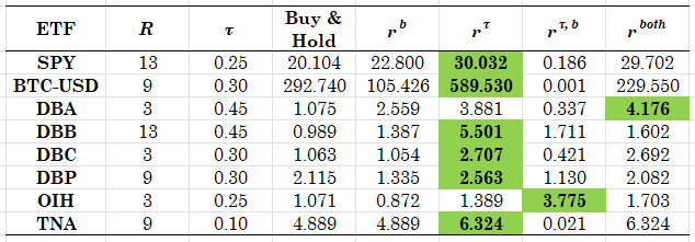
Table 1. Performance of trading strategies for the speculative probabilities - table entries are the NAV of $1 invested in each strategy
As you can easily see from the table, the main strategy based on the "speculative" (and updated) probabilities is excellent in performance - conditional on the correct choice of the threshold [math] \tau [/math] which varies considerably. A cross-validation approach can be used to select this threshold ex-ante, which is something that one can pursue as an exercise or extension of these results. Of note also is the result that the combination strategy that uses both the historical probability estimate and the updating probability estimate works in general very well, while the strategy that works on the comparison of the historical with the updating probability does not work at all - with the exception of the OIH ETF. Similar results hold true for the daily returns and for the trading approach without shorting.
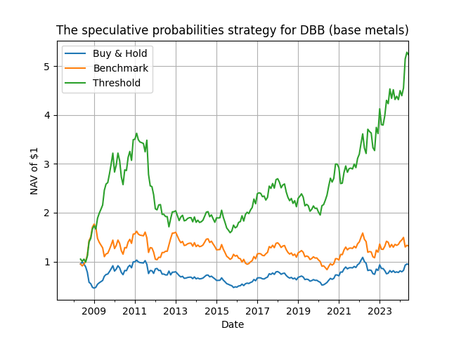
The moral of the story is that simplicity works, and sometimes it can work wonders. Probabilistic strategies offer a number of advantages, and in particular an assessment of risk encapsulated in the probability estimate itself. As you ponder the potential of this set of strategies for your toolbox, have a look at the plot below for the evolution of performance for base metals - not bad for a simple updating rule!

Figure 1. NAV of $1 for the speculative probability strategy vs. the passive buy & hold and the historical probability estimate as the benchmark.


