


By D. Thomakos
As we noted in the last post here , the site is under transfer to a new (and improved) location! We shall be rebranding soon! This is the cause of the small delay in new posts. Be that as it may, I am back with another idea on how to get your returns rolling when your run dry of how to beat the market!
In this post I consider the notion of standardization of a random variable and how this can effect the results of a trading strategy. Consider the returns of an asset [math] y_{t}[/math] and think of another random variable, say [math] s_{t}[/math] everywhere positive and drawn from some distribution independently of [math] y_{t}[/math]. This new random variable acts like a standard deviation in regular standardization but not quite in our case! Suppose, as I do in the implementation, that we have [math]s_{t} \sim U[o, b][/math] and so [math] s_{t}[/math] is uniformly distributed in the interval [0, b] for some upper bound [math] b[/math].
Then, consider the new random variable [math] z_{t} \doteq y_{t}/s_{t}[/math] and compute the first-order autocorrelation of it, i.e., [math] \rho_{z}(1) = \left\{\mathsf{E}(z_{t}-\mu_{z})(z_{t-1}-\mu_{z})\right\}/\sigma_{z}^{2}[/math]. Now, if the scaling by [math] s_{t}[/math] was such that the standardized variable would have small(er) autocorrelation than the original variable we could easily (and safely) predict [math] z_{t}[/math] by its sample mean - and then reverse the standardization and predict [math] y_{t}[/math]! But we still have no idea what the "right" or "appropriate" standardizing variable should be, even with b fixed at some value; but we can do a good job via simulation and resampling, as follows:
Step 1. Generate [math] j=1, 2, \dots, B[/math] samples [math] s_{tj}[/math] of random draws of independent random variables from the [math] U[0, b][/math] distribution of size [math] n[/math], the sample available for [math] y_{t}[/math].
Step 2. Form the standardized variables [math] z_{tj} \doteq y_{t}/s_{tj}[/math] and compute their first-order autocorrelation [math]\widehat{\rho}_{j}(1)[/math].
Step 3. Rank the standardized variables in increasing order of their absolute first-order autocorrelation and select the minimum, i.e., select [math] z_{t(1)} = argmin_{j\in\left\{1, 2, \dots B\right\}}\widehat{\rho}_{j}(1)[/math] and compute its sample mean over a rolling window of [math] R[/math] observations [math]\bar{z}_{t(1)} \doteq R^{-1}\sum_{\tau=t-R+1}^{t}z_{\tau(1)}[/math]
Step 4. Compute the prediction of the original variable as [math] \widehat{y}_{t+1|t} \doteq 0.5\cdot b\cdot \bar{z}_{t(1)}[/math] and trade it to obtain the return [math] r_{t+1|t} \doteq sgn(\widehat{y}_{t+1|t})y_{t+1}[/math]. That's it!
And, you ask, does this approach generate excess returns??! You bet it does, and the results below will certainly illustrate that! In Table 1 below I have collected the backtesting results from a trading exercise with weekly returns over the two years 2022-2023, across various values of the pair [math](b, R)[/math] and [math] B=100[/math] replications (yes, results will change in terms of combinations if you use different values of [math] B[/math], you should try it!). You will immediately note that the method works across different combinations and, therefore, one can devise some form of cross-validation to "optimally" select these parameters - but that's an exercise for the reader. The ETFs that I am using should be standard fare for the readers, and the Python code is always to be found at my github repository.

Table 1. performance attribution of the standardized speculator strategy, total excess returns over the passive benchmark
What is interesting about this approach is that it will work on different random draws of the [math] s_{t}[/math]variable, with different values of the upper bound $latex b$ and different values of the replications [math] B[/math]. The results will differ each time but you will get excess returns and, clearly, you can use either [math] B[/math] to be very large or average across many draws with [math] B[/math] set to a smaller value. Get your hands on the Python code and experiment to find out more! And check Figure 1 below, representative of a different run for Bitcoin as the one above in Table 1, but still speculatively satisfying!
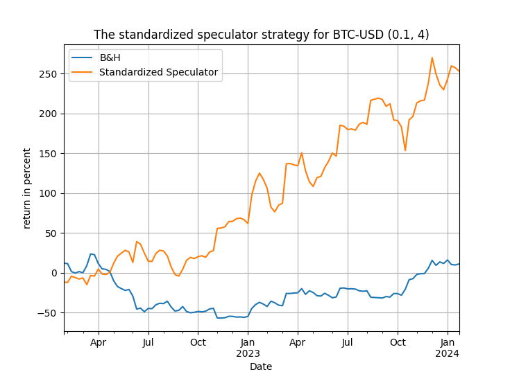
Figure 1. evolution of total trading return for the standardized speculator strategy vs. the passive benchmark, Bitcoin, weekly data from 2022