By D. Thomakos
I recently conducted a poll in LinkedIn about the interplay between "luck" and "skill" in market timing. I got the urge to revisit this favorite topic of mine, market timing, and to see if I could illustrate theoretically that market timing is not only feasible but, importantly, a desirable trading strategy. Ergo, check this short (technical) note in SSRN that illustrates mathematically what most poll respondents answered intuitively: market timing requires both "luck" and "skill" - no doubt about it, the math say so!
A neat implication of the results of the above note is this: even guessing will work better than buy & hold, at least when - and locally in time - there are no equal probabilities of a rising and falling return of any asset. Any local trend makes market timing a priori optimal vis-a-vis the passive benchmark. Furthermore, if guessing is also a viable market timing strategy, then so is any strategy that issues random signals: if we could only find a way that ensures that such randomness will work consistently in our favor then we can certainly build a trading strategy around it. Let me show you one way that this can be done.
The idea is a combination of the signal generator of the lazy moments strategy post and randomized parametrizations. The trick here is to select the parametrizations so as to ensure out-of-sample predictability in a manner that provides consistent out-of-sample financial performance. Here are the prerequisites of the method.
First, let [math] \mathbf{r}_{t}(R) \doteq \left[r_{t-R+1}, \dots, r_{t}\right]^{\top}[/math] denote an [math] (R\times 1) [/math] vector of the last R returns of an asset.
Second, let [math] \mathbf{W}_{j} [/math] denote an (R×B)(R×B)(R×B) matrix of random parameters, for some j=1, 2, ... , J, drawn from the uniform distribution, i.e.,(a,b) [math] w_{\kappa, \ell} \sim U(a, b) [/math] for some [math] a\leq b[/math].
Third, let [math] \mathbf{z}_{tj}(R, B) \doteq \mathbf{W}_{j}^{\top}\mathbf{r}_{t}(R)[/math] denote the [math] (B\times 1) [/math] vector of linear combinations of the random parameters with the returns, that incorporates randomness.
Fourth, apply the lazy moments signal variable as the ratio of the sample mean to the sample median of the components of the vector [math] \mathbf{z}_{tj}(R, B)[/math] and trade. That's it!
However, we need a training procedure for this approach because of the different results one will obtain any time a random matrix is drawn. Here is the simple algorithm that trains this approach to perform well in real-time and real-life: since I attempt to harness randomness, I call the method and the algorithm the random enforcer.
Step 1. Select whether you operate with the original returns or their signs, i.e., whether you use [math]\mathbf{r}_{t}(R)[/math] or [math] sgn\left[\mathbf{r}_{t}(R)\right] [/math].
Step 2. Select the simulation parameters: the range of the uniform distribution [math] (a, b) [/math], the rolling window R, the number of random draws B, the number of replications J. Please see the Python code in my github repository for more information about these parameters.
Step 3. Split your sample to a training and validation set, find the best random parameter structure in the training data (I use averaging also, you can find it in the code!) and retain it for the validation data; perform the validation and examine the results with the parameters that were kept fixed during the validation period. Consider using these parameters for your out-of-sample trading signals.
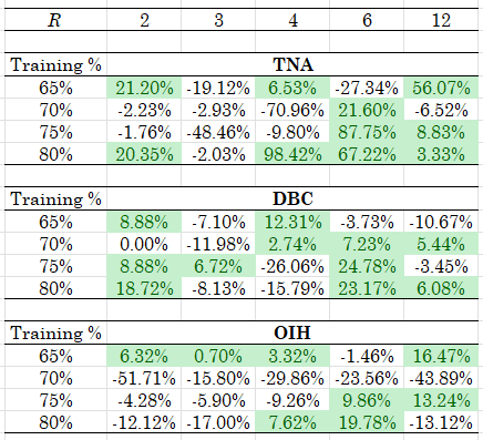
There are a lot of things one can do with this method and, you should experiment to find this out, you can get some truly robust and profitable parametrizations. In fact, in most of my experiments the random enforcer produced excess returns vs. the passive benchmark that justify its a priori use. Table 1 below showcases a representative run for three highly volatile ETFs: TNA (my leveraged favorite), DBC and OIH - you should think of volatile assets as your friends in trading strategies such as this one! The data are weekly returns and the start from 2019 - you can easily get more results using the Python code and adapting it to your liking!

Table 1. Performance of the "random enforcer" strategy, weekly rebalancing, results are excess returns in percent (strategy minus the passive benchmark) and are for the a delay parameter of 2 weeks, across several rolling windows R for that delay and training periods. For these results we set J=3 and B=5 and the range of the uniform distribution is U(-1, 1).
Can you make some speculative returns using the random enforcer? Oh yes, you can and you should - don't let randomness fool you: maybe the trend can be your friend but its volatility and chance that will make your money dance!


