By D. Thomakos
I am always fascinated by financial assets that are "bubbly" and highly non-stationary because of their increased volatility. They are great for speculation, if you can manage the large swings and the large drawdowns that they have, but they have something that makes them unique. So, in this post I am exploring the return-volatility nexus for some highly volatile and highly speculative assets - and read on, you will not be disappointed!
Let us start with some definitions. Let [math] r_{t}[/math] denote the percent return of our asset of interest and let [math]v_{t} \doteq \vert r_{t}\vert[/math] denote the absolute return which acts as a volatility proxy (see this past post on this relationship). If volatility is a driver of future returns, we should be able to use it successfully in trading - for it makes sense that, for highly volatile assets, past volatility in an upswing, for example, will be followed by volatility in a downswing; and there has to be such a cycle of upward and downward price movements otherwise the asset will not be volatile, right? The idea then is simple: here are the steps for its implementation.
Step 1: For a fixed window of [math]R[/math] observations compute the cross-correlation [math] \widehat{\rho}_{rv}(d)[/math] between the pair [math](r_{t},v_{t-d})[/math] for values of [math]d = 1, 2, \dots, d_{\max}[/math].
Step 2: Compute and store the delay of the maximum and minimum cross-correlations, and also of the corresponding maximum and minimum absolute cross-correlations i.e., find [math]d_{1}^{*} \doteq argmax_{d} \left\{\widehat{\rho}_{rv}(d)\right\}[/math] and similarly find [math]d_{2}^{*} \doteq argmin_{d} \left\{\widehat{\rho}_{rv}(d)\right\}[/math], and then repeat for the absolute cross-correlations i.e., [math]d_{3}^{*} \doteq argmax_{d} \left\{\vert \widehat{\rho}_{rv}(d)\vert \right\}[/math] and [math]d_{4}^{*} \doteq argmin_{d} \left\{\vert \widehat{\rho}_{rv}(d)\vert \right\}[/math].
Step 3: Construct 4 trading rules based on the change of volatility at the "optimal" delays as above, that is use the signal variables [math] s_{tj}(q) \doteq \Delta v_{t-d_{j}^{*}+q}[/math] for [math]q = \left\{0, 1\right\}[/math] i.e., use the optimal delay as is computed or one-period forward. Trade with [math] \widehat{r}_{t+1|t,j}(q) \doteq r_{t+1}\cdot sng(s_{tj})(q)[/math].
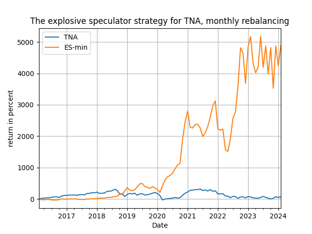
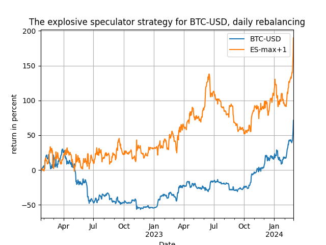
That's it, and my claim now is this: there is at least one value of [math]d_{\max}[/math] and at least one of the signal variables [math]s_{tj}(q)[/math] that will provide a very significant over-performance over the passive benchmark. You can always experiment more with the Python code available from my github repository. I will be illustrating this trading method using three very volatile assets, OIH (oil services ETF), my favorite TNA (3x leveraged small cap ETF) and, of course Bitcoin. The results are for daily rebalancing (2022-01-01 to 2024-02-29) and for weekly and monthly rebalancing (2014-01-01 to 2024-02-29) - please note that because different values of the initial window [math]R[/math] are used in different frequencies the results of the passive benchmark will naturally differ.
Table 1: performance attribution of the explosive speculator strategy
Now if these ain't explosive results I don't know what they are! You can clearly see that in all, but one, cases the explosive speculator strategy significantly outperforms the passive benchmark - and this is true even when the passive benchmarks performs really well (or really bad, doesn't matter!). Clearly there is merit in the strategy and you should research it further, for it can be automated even more - but that's for you to find out how! Correlation, therefore, works wonders if one knows which variables to correlated with. Stay tuned and check to representative cumulative return plots below!