By D. Thomakos
The summer in Greece is not really conducive to research activities but, I must stress this, the relaxation is conducive for generating ideas! This post is such an idea, born out of a long dive in the beautiful seas around the town of Nafplio in the Peloponnese and the beach at Kondyli. And the idea was very simple: in the marketplace, especially in a bull run that everyone is optimistic, the most common benchmark is the buy and hold strategy. This strategy implies a forecast for next trading period of +1, just buy - buy and buy again and stay with your chosen asset. What if, then, we take +1 as the main forecast and change it based on some condition on market performance? This idea is essentially one that takes a simple forecasting model and fixes its constant term at +1 and is built around that particular premise above.
Let's see this in math terms. We first define [math] y_{t+1} \doteq sgn(r_{t+1}) [/math] as the actual sign of the returns, [math] y_{t+1|t} [/math] as the forecasted sign of the returns and then we write our forecasting model as [math] y_{t+1|t} \doteq 1 - \gamma I(z_{t} < 0)[/math] where [math] \gamma [/math] is a parameter and [math] I(z_{t} < 0) [/math] is an indicator function based on past returns. For example, and this is what I used in the application, you may define [math] z_{t} [/math] as [math] z_{t} \doteq r_{t-d}[/math] or as [math]z_{t} \doteq \sum_{j=t-M-d+1}^{t-d}r_{j}[/math]; [math] M[/math] here is a rolling window to compute the indicator and [math] d [/math] is the delay. In all cases you create a dummy variable with a condition that will trigger a reduction to the value of the benchmark forecast of +1. The parameter or as [math] \gamma > 0[/math] is, as I shall show next, always positive.
The parameter [math] \gamma [/math] is easily estimated from the relationship [math] \mathbb{E}(y_{t+1}) - 1 = -\gamma \mathbb{E}\left[I(z_{t} < 0)\right][/math]. Since both the right-hand and left-hand side expectations are for binary variables they are equal to their respective probabilities and I can write [math] \gamma \doteq \left\{\mathbb{P}(y_{t+1}=+1) - \mathbb{P}(y_{t+1}=-1) - 1\right\} / -\mathbb{P}(z_{t} < 0)[/math] which simplifies to [math] \gamma \doteq 2\mathbb{P}(y_{t+1}=-1)/ \mathbb{P}(z_{t} < 0)[/math], which is always positive.
What is interesting is that the value of [math] \gamma [/math] becomes a constant and equal to 2 in the particular choice of [math] z_{t} = r_{t-d}[/math]. Then we can write [math] \gamma \doteq 2\mathbb{P}(y_{t+1}=-1) / \mathbb{P}(y_{t-d} = -1)[/math] which under stationarity reduces to [math] \gamma = 2[/math]!
Substituting sample moments, possibly over another rolling window [math] R [/math], for the theoretical moments above one can estimate [math] \gamma [/math] for any choice of the [math] z_{t} [/math] variable. Its as simple as that and, naturally, we are ready to go to the application. The parameters of choice are [math] (d, M, R) [/math] and the I will use the two indicators for [math] z_{t} [/math] as described above. Four strategies will be tested:
S1, will use the [math]z_{t} = r_{t-d}[/math] indicator and the forecast will be [math] y_{t+1|t} = 1 - 2 I(r_{t-d} < 0)[/math]
S2, will use the [math] z_{t} = \sum_{t-M-d+1}^{t-d}r_{j} [/math] indicator and the forecast will be [math] y_{t+1|t} = 1 - 2 I(z_{t} < 0)[/math], i.e., it will not use the estimated [math]\gamma[/math] parameter.
S3, will be like S1 but it will use the estimated value of the [math] \gamma[/math] parameter and the forecast will be [math] y_{t+1|t} = 1 - \gamma I(r_{t-d} < 0)[/math] .
S4, will be like S2 but it will use the estimated value of the [math] \gamma[/math] parameter and the forecast will be [math] y_{t+1|t} = 1 - \gamma I(z_{t} < 0)[/math].
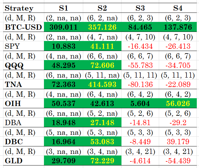
I will present results for a number of ETFs, based on daily rebalancing and for the period after 2022. In the Python code that you can find in my github repository you can experiment with other rebalancing frequencies as well - the method does work for weekly and monthly rebalancing with appropriate reparametrizations. The results are for the ex-post optimal values of the parameters which are obtained via direct search. Table 1 below has the results.

Table 1. Total excess returns, over the buy and hold benchmark, from the use of the 4 strategies. The best ex-post parameter combinations are shown. Daily rebalancing with the data starting in 2022.
The results are speculatively conclusive! Not only does the idea works but it works well without the need of estimation of the parameter [math] \gamma [/math]. The best strategy is S2, followed by the simpler S1. Notable exceptions where all strategies work are the Bitcoin and the OIH, for the latter having the S4 as the top performing strategy. The excess returns are considerable to ignore these strategies from your toolbox!
There you have it: a simple, easy to train and implement, quantitative trading strategy coming out straight from the summer vacations. Grab the Python code and make the summer's ending speculatively memorable!


