By D. Thomakos
History is a never-ending source of inspiration, and humility. It teaches us not only to appreciate what has been done before us but also how to improve upon it. In this post I am taking my historical que from a 1937 paper of Alfred Cowles and Herbert E. Jones titled "Some A Posteriori Probabilities of Stock Market Action". The main theme of the paper is runs and reversals and their interaction in financial markets. This particular paper is important for two reasons: first, so many-many years back it contains an analysis of financial data across many frequencies starting with 20 minutes! second, it considers the runs-to-reversals ratio as an indicator of stock market predictability. It is this second contribution that gives the inspiration for this post. Runs are simply sequences of the same sign, in our context are sequences of successive positive or negative returns; reversals are obviously the times when the market changes direction and the runs-to-reversals ratio (R2R in what follows) is an indicator of non-randomness in the market. The idea of using runs to check randomness of data is old, see for example this entry in Wikipedia for the Wald-Wolfowitz runs test or this original article here. There is also this follow-up randomness test of the same authors based on series correlation which I found while writing this article, and on which I might return in another post - add it to your references!
Runs are easy to compute and getting the R2R ratio is easy to compute too. If this is of any usefulness as a trading indicator it will show-up in the data - and it does in a spectacular way for assets that are mostly volatile, as those that we have examined in the last post of the explosive speculator. So let's see what the signal variable is and how to trade the R2R strategy! Let [math] Q_{t}(w)[/math] denote the R2R ratio computed over a window w of observations around time t, i.e., [math] w\in \left\{t-w+1, t-w, \dots, t\right\}[/math]. Define the signal variable relative to a threshold [math]\alpha > 0[/math] of the size of the R2R ratio, that is define:
[math] s_{t+1|t}^{R2R} \doteq I\left[Q_{t}(w) > \alpha\right]-I\left[Q_{t}(w) \leq \alpha\right][/math]
and then use this signal variable to trade as usual, i.e., the trading returns of the R2R strategy are given by:
[math] r_{t+1|t}^{R2R} \doteq s_{t+1|t}^{R2R} \cdot r_{t+1}[/math]
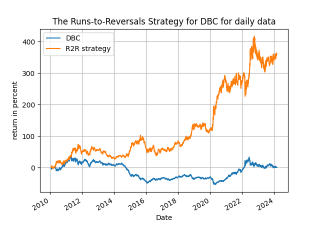
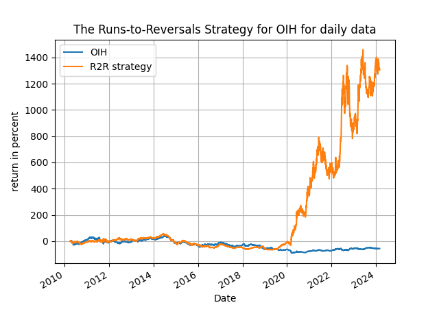
where [math] r_{t+1} [/math] are the percent returns of the asset under consideration. As usual the choice of the parameters [math] (w, \alpha)[/math] is what determines performance but you can easily find ways to optimize them in a real-life application. The results that follow are illustrative of the power of this particular indicator and you will be speculatively surprised by them! In the Python code that you can find in my github repository you can experiment with different assets, different frequencies and different parameter combinations very easily. In the table below I show performance using daily data with two different starting periods, from 2022-01-01 to 2024-02-29 and from 2010-01-01 to 2024-02-29 for just four very volatile assets: the OIH, DBC and TNA ETFs and the Bitcoin. You can get very good results with other assets too, including commodities and the market when trending, as well as different frequencies, but you have to find this on your own! Have a look now at the results in Table 1:
Table 1: performance attribution of the R2R strategy
As you can see the results are mighty speculative, sometimes better and sometimes not as explosive as in the previous post - but the point is that you can actually use the R2R ratio as your trading indicator - because it works! The market can be timed and is your duty as a speculator to find out the many ways that this can be done so, run little trader, run!


