


By D. Thomakos
This is our inaugural post in the new Prognostikon site, so let's kickstart it with something new and exciting! A recurrent theme in economic policy analysis and quantitative trading strategies is that of the impact of uncertainty in macroeconomic variables, currencies and global commodities. There is considerable research, academic and professional, as to how one can use macroeconomic conditions to forecast currencies and commodities and create quantitative trading strategies based on these conditions. In this post I offer such a strategy that combines policy uncertainty with currency and commodities trading - it's simple and works very well, so read on!
I start by considering the economic policy uncertainty indices of Baker, Bloom and Davis, see their site here, which are available for direct online download from the FRED database. In the past I have used the Global Economic Policy Uncertainty Index to perform long-term wheat forecasting, see this past post. Now, I take some particular countries and their corresponding indices to construct a simple index of my own. These countries are the United States, the United Kingdom, the European Union, India and Russia. The selection of these countries should be self-explanatory, but you can always disagree, and you can change them if you get your hands on the Python code in my github repository! The index is the plain average of the scaled individual indices.
Let [math] x_{tj}[/math] denote the index of the jth country and let [math]u_{tj}\doteq x_{tj}/x_{0j}[/math] denote the scaled index. My global uncertainty index (GUI) is then defined as:
[math] G_{t}^{UI} \doteq 0.2 \sum_{j=1}^{5}u_{tj}[/math]
I next link this index to a selection of currency and commodity ETFs, the following ones:
- The currency ETFs for the euro-US dollar exchange rate FXE, for the British pound-US dollar exchange rate FXB, for the Japanese yen-US dollar exchange rate FXY, for the Swiss franc-US dollar FXF and for the Australian dollar-US dollar FXA.
- A currency basket ETF vs. the US dollar UUP.
- Commodity ETFs for agriculture DBA, for general commodity tracking DBC, for oil services OIH and for wheat WEAT.
All data are transformed to their monthly growth rates and I thus define as my explanatory variable the monthly growth rate of the GUI index [math]z_{t} \doteq \Delta \log(G_{t}^{UI})[/math] and as my dependent variables the monthly returns of the above ETFs [math]y_{tj}\doteq \Delta \log(P_{tj})[/math], where [math] P_{tj}[/math] is the monthly closing price of the respective ETF j. Note that in my trading evaluations I will use the percent returns not the log-returns! My analysis will have three parts: (a) the identification of the lead-lag relationship between the ETFs and the index, [math] (y_{t}, z_{t-d})[/math], (b) the use of this lead-lag relationship to offer a simple, delay-based, forecasting model for the monthly returns of the ETFs, [math] \widehat{y}_{t+h} \doteq \widehat{\alpha} + \widehat{\beta}z_{t-d+h}[/math] and (c) a simple trading exercise whereas the past signs of the GUI index will be used to trade the ETFs. You can find details of parts (a) and (b) in the Python code so I will not discuss them further here - but you should look at them to make the connection between the lead-lag relationships, the forecasts that you can easily generate and the trading results, on which I will go immediately next!
Let then [math] r_{t+1,j} \doteq \exp(y_{t+1,j})-1[/math] be the actual next period percent return of the jth ETF and let [math] s_{t-d} \doteq \exp(z_{t-d})-1[/math] for values of the delay parameter between 0 and 11 months, [math] d=0, 2, \dots, 11[/math]. I trade the ETFs by the simple rule:
[math] \widehat{r}_{t+1,j}^{UI} \doteq r_{t+1,j} sgn(s_{t-d})[/math]
The results in Table 1 below indicate the optimal delay [math] d [/math] for each ETF and the total trading return over its respective evaluation period (please see the Python code for details):
Table 1. Performance attribution of the GUI strategy vs. the passive benchmark, monthly data
The results from Table 1 are speculatively good! As you can see, for all ETFs (save the UUP currency basket one) have excess returns many times over their corresponding passive benchmarks, and in some cases as in OIH or DBC or WEAT the results really blazing! It is clear that one can very profitable consider the economic uncertainty indices as good macroeconomic signals for trading currencies and commodities. In Figures 1 and 2 we showcase the evolution of total trading returns for the FXB and WEAT ETFs and you can easily see the usefulness of the index signals.
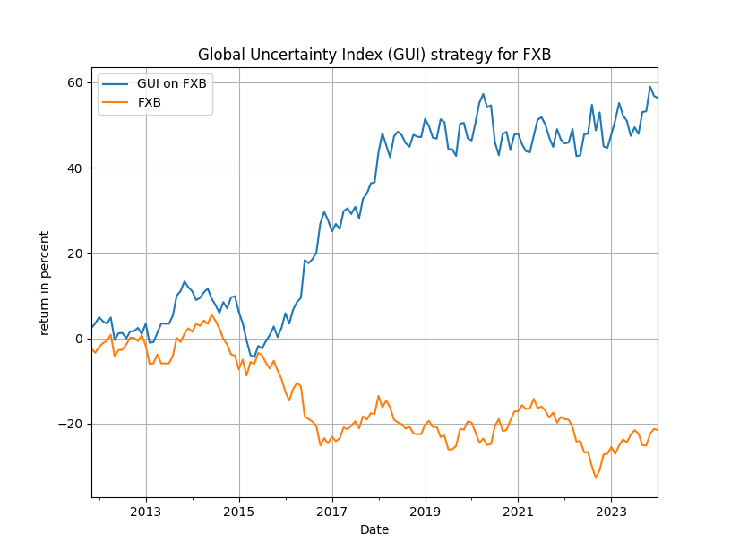
Figure 1. Total trading return for the GUI strategy vs. the passive benchmark FXB, British pound to US dollar
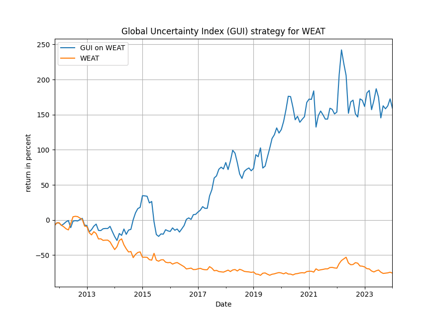
Figure 2. Total trading return for the GUI strategy vs. the passive benchmark WEAT
You can easily experiment more with the same data or adapt them to your particular needs, but what is the take-away message from these results is that there is critical and useful information in the uncertainty indices, certainly in the GUI index used here, and further research can reveal how we might make additional use of the same data for forecasting and trading. I might return to them in a follow-up post.