


By D. Thomakos
Yep, this is another one of them posts that take a little-known historical piece of financial innovation and turns it into a practical strategy for today! Enter L. C. Wilcoxen's 1942 paper "The Market Forecasting Significance of Market Movements, published in the Journal of the American Statistical Association. To the best of my limited historical knowledge, this is the first paper that I am encountering to have a full-fledged backtesting of a trading strategy - this is the figure that you see in the beginning of this post!
What was the idea of Wilcoxen that I am trying to replicate and expand here? It is about "market cycles", and he has quite an innovative approach for finding them (for the understanding of his time that is!) The gist of Wilcoxen's approach is to work with non-overlapping intervals of certain days length and to trade them based on some signaling condition. I have not replicated Wilcoxen's method exactly but have taken a different route to exploit the idea of such "market cycles". Here is what I did.
First, I start with the an interval of length $latex \tau$-days and compute the total return of an asset over that interval, like in the following:
[math] R_{t_{j}}(\tau) \doteq \prod_{s=t_{j}-\tau+1}^{t_{j}}(1+r_{s})-1[/math]
where [math] r_{t}[/math] is the daily return of the asset and where [math] t_{j} \doteq t_{j-1} + \tau[/math] for [math] j=2, 3, \dots, \left[n/\tau\right][/math] defines the non-overlapping intervals of length [math] \tau[/math] in a time series of size [math] n[/math]. Here the notation [math] \left[n/\tau\right][/math] denotes the smallest integer of such intervals available for backtesting. Then, I define my signaling variable which I found after some experimentation. This is the sign of the 3rd quartile of the last 5 such non-overlapping intervals - don't ask me why it works, you can come up with explanations and easily adjust the Python code available in my github repository! I write the signaling variable as:
[math] S_{t_{j}} \doteq sign\left[Q_{3}(R_{t_{j}},R_{t_{j-1}}, \dots, R_{t_{j-4}})\right][/math]
with corresponding trading return over the next non-overlapping interval equal to:
[math] R_{t_{j+1}}^{SC} \doteq R_{t_{j+1}}\cdot S_{t_{j}}[/math]
where the notation of $latex SC$ stands for the speculative cycle strategy! Now, how does one backtest such a strategy? The possible intervals are many and direct search is not really an option here, so I follow a different approach. I split my sample into training and testing periods and for the training period I do the following, over a number of $latex K$ assets; the first 4 steps are for the training sample and step 5 is for the testing sample.
1) For a sequence of intervals [math] \tau \in \left\{\tau_{\min}, \dots, \tau_{\max}\right\}[/math] compute the total trading return of the passive benchmark and the speculative cycle strategy i.e., compute [math] R_{\left[n/\tau\right]} \doteq \prod_{j=1}^{\left[n/\tau\right]}(R_{t_{j}} +1)-1[/math] and correspondingly compute [math] R_{\left[n/\tau\right]}^{SC} \doteq \prod_{j=1}^{\left[n/\tau\right]}(R_{t_{j}}^{SC} +1)-1[/math].
2) Compute the excess return of the strategy over the benchmark i.e., [math] E_{\left[n/\tau\right]}^{SC} \doteq R_{\left[n/\tau\right]}^{SC}-R_{\left[n/\tau\right]}[/math] and store it along with the value of [math] \tau[/math].
3) Repeat the above steps for all [math] K[/math] assets available.
4) Compute the quartiles of the values of [math] \tau[/math] across all [math] K[/math] assets for the top 3 performing values of [math] \tau[/math], thus generating a new sequence of 9 "optimal" [math] \tau^{*}[/math] values.
5) Take this new sequence of [math] \tau^{*}[/math] values and apply it in the testing sample, report results.
What is interesting in the above approach is that I aggregate the "cycle" lengths [math] \tau[/math] across assets, because if there is a "market cycle" it should not differ that much from one asset to another (or maybe it does? what do you think?) The testing results are quite encouraging and are summarized in the figure below (note that training is for daily data until 12/2020 and testing for the last 3 years i.e., from 01/2021 until 12/2023).
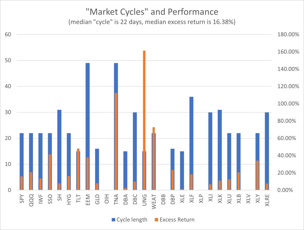
Figure 1. "optimal market cycles" and performance as excess return over the passive benchmark; "cycle" length measured on the left axis, excess return mea
The median of the "optimal cycle" is about one month, at 22 days, and you can see that many of the assets in the list of ones being examined have "cycle" lengths that are close to the median - of course there are some higher and some lower. What is even more interesting is that from among this list of 27 assets only 4 (15%) do not have positive excess returns (but with some adjustments they can too!). Furthermore, 9 out of 27 assets (33%) have "cycle" length equal to the median of 22 days and 14 out of 27 assets (52%) have a "cycle" length equal to either 22 or 30 or 31.
Are "market cycles" for real? If you believe so grab the Python code and experiment yourself to find out more! For the time being you have another quantitative strategy whose origins go back to 1942 when L. C. Wilcoxen tried to answer the same question!