By D. Thomakos
Welcome to the last (technical) post of 2023! This is going to be the first part of a two-part series on echo-state networks (ESN). This is type of a recurrent neural network (RNN) that is most suitable for time series analysis tasks, such as smoothing and forecasting, and is characterized by its simplicity of construction, robustness and linear training method. Thus, it is fast and can be a very useful, and highly competitive to other approaches, model in your time series toolbox. Unfortunately, going over the theory and the math is beyond the scope of this post, but you can easily get very good summaries and working code from the originator of this type of network Herbert Jaeger, see for example here, and from Mantas Lukoševičius webpage here. The Python code that you will find in my github repository is adapted from Mantas' publicly available code with many thanks.
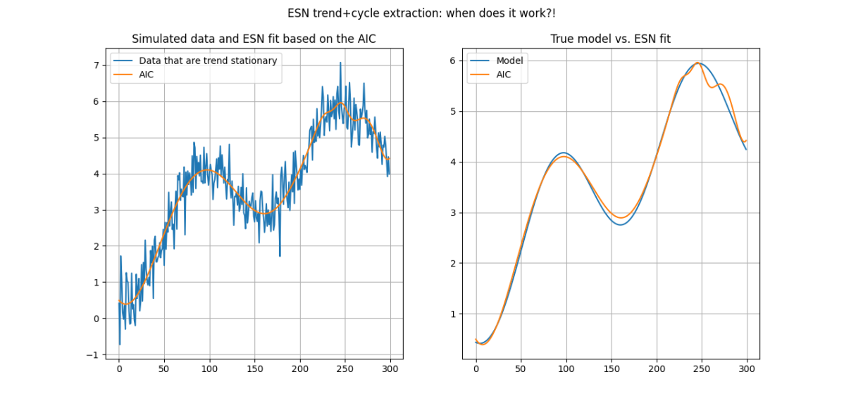
Now, the original idea for using the ESN was to generate, well, speculative returns! But that is going to be the second part of this series (and hopefully the first post for 2024!). In this post I am taking my cue from a different set of considerations which are well-known in the econometric time series literature and were aptly repeated in this LinkedIn post by Valeriy Manokhin. I will be using the ESN as a smoother and trend extraction method and will be illustrating how it can be used for exploratory data analysis (EDA) but also for understanding the type and complexity of a time series. The good thing is that we can learn a lot from simulating time series and applying the ESN to them, and this is what I will be doing in this post.
Let [math] y_{t}[/math] be a time series of interest. I shall differentiate between two cases of a data-generating process: first, a trend-stationary time series and, second, a difference-stationary time series. Both these cases can be written in model form as:
[math] y_{t} \doteq f_{t}(\theta) + \eta_{t}[/math]
where [math] f_{t}(\theta)[/math] is the trend (plus cycle if desired) function (or "model") and where [math] \eta_{t}[/math] is the error or noise; here [math] \theta[/math] denotes a vector of parameters that we would be estimating - if we knew the functional form of [math] f_{t}(\theta)[/math], but we don't!. When we are dealing with a stationary series then [math] \eta_{t} \doteq \epsilon_{t}\sim WN(\sigma_{\epsilon}^{2})[/math] but when we are dealing with a non-stationary series then [math] \eta_{t} \doteq \sum_{\tau=1}^{t}\epsilon_{\tau}[/math]. The definition, or nature, of the noise variable is crucial in understanding what we can and cannot achieve when attempting smoothing and trend extraction with ESN (or any other method for that matter!).
The ESN is built on the idea that complexity can be "harnessed" through multiple network connections of a "state" variable (to be constructed) with random weights, and the dimension of the state variable (as a vector) will determine (along with any input variables that we may have) the ability the network to reproduce signals or to perform other tasks such as smoothing and forecasting. The mathematics of the ESN are neat, the representation is also neat, the construction of the state variable straightforward and the training of the network is just a linear regression. The code required is compact and fully explainable and the ESN is a very robust way to parametrize complexity, and thus to represent it efficiently.
There is a plethora of methods for approximating [math] f_{t}(\theta)[/math] and you can easily find them in a quick literature or internet search. Here I shall illustrate how you could do this by combining the polynomial basis of Chebyshev polynomials with the power of an ESN - and I will do this by utilizing a natural property of the ESN: the dimension of the output training weights is the dimension of parametric complexity of the network and, thus, we can immediately use a model selection criterion, such as the AIC or the BIC, to select the complexity dimension of the ESN that is best suited for purposes of trend extraction and smoothing.
Thus, first I will construct my "explanatory" variables via the Chebyshev polynomial basis and put them into the vector [math] \mathbf{x}_{t}[/math]. A low-order basis is required so the dimension of [math] \mathbf{x}_{t}[/math] will not be greater than 2 or 3 - but you can always experiment for your particular data. Then, I will feed my data [math] \left\{y_{t},\mathbf{x}_{t}\right\}[/math] into the ESN, construct the state variable over a range of dimensions [math] s=s_{\min}, \dots, S_{\max}[/math] for some [math] s_{\min}[/math] that can be as low as 2 to some [math] S_{\max} >> 0[/math]. Let [math] \mathbf{z}_{t}(s) \doteq \left[\mathbf{x}_{t}, \mathbf{s}_{t}\right]^{\top}[/math] denote the concatenated vector of the input variables and the state variables [math] \mathbf{s}_{t}[/math], a vector of dimension [math] (s \times 1)[/math]. It is important to stress here that [math] \mathbf{s}_{t}[/math] is a function of [math] \mathsf{s}_{t-1}[/math] and a set of random weights that fully connect the components of [math] \mathbf{s}_{t}[/math] with [math] \mathbf{s}_{t-1}[/math], with [math] \mathbf{x}_{t}[/math] and with [math] y_{t}[/math]. Once the [math] \mathbf{z}_{t}(s)[/math] vector is available for [math] t=1, 2, \dots T[/math], then the output weights [math] \mathbf{W}^{out}(s)[/math] are trained by linear (regularized) regression on the time series [math] y_{t}[/math]. The fitted values from this procedure, for a selected value of [math] s[/math], correspond to the approximation [math] \widehat{f}_{t}(s)[/math] of the unknown "model" [math] f_{t}(\theta)[/math]. Denoting by [math] \widehat{\eta}_{t}(s)[/math] the in-sample residuals from the fitting, I select the degree of complexity [math] s[/math] via the application of any model selection criteria; and this approach works very well:
[math] s^{*} \doteq argmin_{s\in \left\{s_{\min},S_{\max}\right\}} T\log\left(\widehat{\sigma}_{\widehat{\eta}(s)}^{2}\right) + P(s,T)[/math]
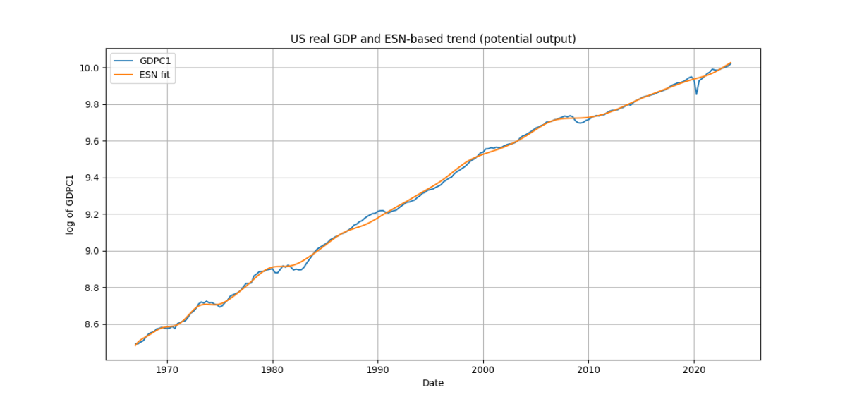
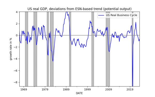
where [math] P(s, T)[/math] is the penalty factor according to the criterion used. You can learn or lot for the nature of a time series just by tweaking the parameters in the Python file that accompanies this post. If you aim is to smooth your time series or to understand its low-frequency components or to extract a presumed deterministic component, the simulations show that you can't go wrong with the application of this ESN-based approach. Furthermore, and you can link this to earlier posts on smoothing from the blog, this approach offers you an immediate way to project the extracted "model" component forward at any horizon [math] h > 1[/math] very easily; this is because the input variables are just polynomials in time and, importantly, because you can easily project the state variable [math] \mathbf{s}_{t+h}[/math] as well! Thus, the ESN can be used as a tool for tasks such as extracting potential GDP or core inflation, or any other low-frequency component of a time series. At this stage of my thinking, I have not considered the separation of trends and cycles - but maybe this is something you can do as an exercise!
Get your hands on the Python code and experiment to your heart's content! I am only showcasing two examples as figures below, but there is a lot to be learned by understanding the fundamentals of time series EDA and trend extraction. Do notice the good job that the ESN-based smoothing does in getting the US business cycle right! I hope to offer more applications soon.
Till then, all the best wishes for a happy, healthy and productive (and speculatively profitable!) 2024!!


