By D. Thomakos
I have repeatedly stressed in my posts the need for simplicity and interpretability when constructing quantitative trading strategies. The use of sectoral information when trading an index is not only economically meaningful but also highly interpretable. Different sectors are affected in various ways by economic conditions, and shifts in investor sentiment with respect to sectors will be reflected into the index the sectors participate to. In this post I consider the sectoral ETFs that are available for the S&P500 ETF and work with a very simple trading context that contains, however, an eminently useful twist! My data will be daily returns of the SPY ETF, that corresponds to the S&P500, and these available sectoral ETFs: XLC (communications sector), XLY (consumer discretionary sector), XLP (consumer staples sector), XLE (energy sector), XLF (financial sector), XLV (health care sector), XLI (industrial sector), XLB (materials sector), XLK (materials sector), XLU (utilities sector) and XLRE (real estate sector). The common starting date of the total dataset is 2018. You can easily see that these sectoral ETFs cover most, if not all, of regular economic activity.
The sectoral ETFs act as factors on the index and one can envision a predictive model whereas the returns of the index are regressed on the (lagged) returns of the sectors and a trading strategy is based on the predicted sign of this model. However, and you can experiment by altering the Python code available in my github repository, this idea will not work on its own for various reasons ranging from collinearity, to non-robust estimation, no model reduction, choice of rolling window etc. But none of these reasons is as important as the following one: the nature of the data being used. Let me clarify this. Assume that [math] y_{t}[/math] is the daily return of the index and that [math] x_{tj} [/math] is the daily return of the jth sectoral return, for j = 1, 2, ..., K. A regression model based on this data will read as in:
[math] \mathbb{E}(y_{t}) = \beta_{0} + \sum_{j=1}^{K}\beta_{j}\mathbb{E}(x_{t-1,j}) [/math]
where I intentionally use unconditional expectations (you will see why below). This regression model links the expected returns of the index with those of the sectors - pretty standard staff, right? But the predictive power of such a model is already known to be relatively weak and this is because of the natural properties of returns (not much of persistence in them). But what happens if you convert your data from continuous to discrete for both the dependent and the explanatory variables? Let now [math] s_{t}\doteq sgn(y_{t})[/math] denote the sign of the returns of the index and, correspondingly, let [math] f_{tj} \doteq sgn(x_{tj})[/math] denote the sign of the returns of the jth sector. In this case we can easily see that the expectations in the previous equation become probability differentials since [math] \mathbb{E}(s_{t}) \doteq \mathbb{P}(s_{t} > 0) - \mathbb{P}(s_{t} \leq 0)[/math] and, correspondingly, [math] \mathbb{E}(f_{tj}) \doteq \mathbb{P}(f_{tj} > 0) - \mathbb{P}(f_{tj} \leq 0)[/math]. Therefore, the regression model can now be written as:
[math] \mathbb{P}(s_{t} > 0) - \mathbb{P}(s_{t} \leq 0) = \theta_{0} + \sum_{j=1}^{K}\theta_{j}\left\{ \mathbb{P}(f_{t-1,j} > 0) - \mathbb{P}(f_{t-1,j} \leq 0)\right\} [/math]
which has a completely different interpretation from the standard form. Now the model is about the "strength" of the direction of the dependent and the explanatory variables and direction is (also well known) more persistence than the returns themselves. The use of discrete data in the form of signs alters both the interpretation of the model and the nature and properties of the data entering it. As a reult the predictive ability of the model changes as well - and for the better.
While it is true that this form of a model, with discrete rather than continuous variables, should not be strictly speaking estimated by least squares, in a trading strategy one does not care so much about the properties of the estimators but about the quality of the corresponding forecast the model produces. If you can get good forecasts from least squares so be it! However, with many explanatory variables (here we have 11) one has to be careful a bit more. Thus, I am using hte following parametrization to estimate my probability differentials model: (a) the parameters are estimated using robust regression, (b) the rolling window is fixed to 14 daily observations and (c) I perform two rounds of sequential model reduction for p-values of 90% and 80%. Once the parameters are estimated the forecasted sign of the probability differential gives the sign of the trading direction, i.e., we have:
[math]\widehat{y}_{t+1|t} \doteq y_{t+1}\cdot sgn\left\{ \widehat{\mathbb{P}}(s_{t+1|t} > 0) - \widehat{\mathbb{P}}(s_{t+1|t} \leq 0)\right\} [/math]
I am illustrating the excellent performance of this approach with some results below. The table has the total return of the "speculative sectors" strategy vs. the passive benchmark of the index, and the results are indeed telling! Have a look.
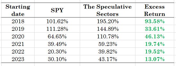
Table 1. Results of the speculative sectors strategy, 14-day estimation window, robust regression with sequential model reduction, daily data
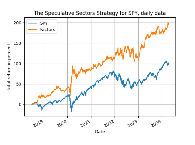
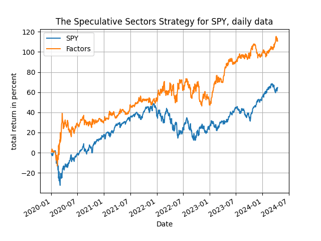
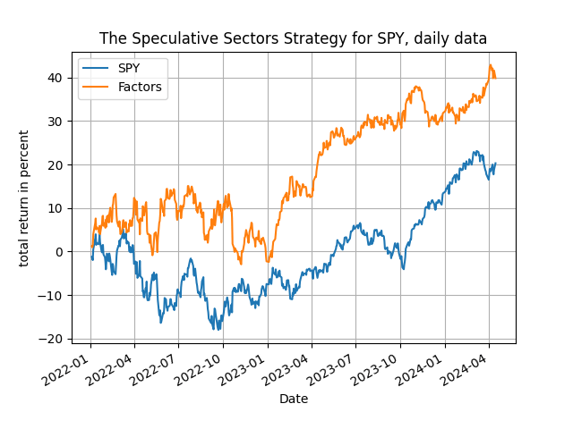
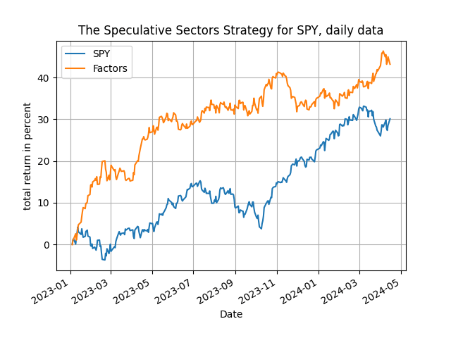
The speculative sectors strategy works uniformly well, with the same parametrization across all starting years that include both an upside and a downside market. The same model is used throughout and therefore we find strong predictability that is practically useful. The strategy outperforms the passive benchmark all the time easily, generating excess returns that range from 20% to 93.5% - not bad for a regression forecast! But you see the trick, the twist, is in the data transformation and in the model interpretation - and you should have already noticed that the use of discrete data both simplifies the model per se and improves performance, while at the same time maintaining a high degree of interpretability. Of course one can monitor which sectors enter significantly in these calculations by adapting the provided Python code, thereby increasing the informational content of this approach.
One last thing. Have a look at the plots of the cumulative returns of the strategy below, from 2018, 2020, 2022 and 2023: the speculative sectors strategy starts off and stays above the benchmark index for the whole period of trading, a good sign of robustness of the method. So, there you have it: sectoral information is useful and you can harness it with ease, go get the Python code and increase your speculation proficiency!
