


By D. Thomakos
Welcome to our pre-Christmas special! In this post I will explore an adaptation of the Bayesian average. I have minimal exposure to Bayesian methods, apart from the wonderful work of Abraham Wald on decision theory - Wald's general result, the complete class theorem, on decision making is Bayesian and Wald himself has acknowledged this! An interesting paper on Wald's complete class theorem is Kuzmics, 2017.
The idea of this post is, however, way simpler and - importantly - is in the same vein of previous posts, i.e., it rests on conceptual simplicity. The simplest forecast I have used for predicting financial returns is the sample mean, usually on a rolling window of [math] R[/math] observations, i.e., [math] \widehat{\mu}_{t|t-1}(R) \doteq R^{-1}\sum_{\tau=0}^{R-1}y_{t-\tau}[/math], where [math] y_{t}[/math] denotes either the continuous return or the binary indicator of positive or negative returns. Let us consider then [math] y_{t}\in\left\{0, 1\right\}[/math] denote the binary representation of the returns and note that the Bayesian estimator of the mean of such a process, under assumptions that you can find for example here in equation (7.4.10), is given by:
[math] \widehat{\nu}_{t|t-1}(R) \doteq \left[\alpha + R\widehat{\mu}_{t|t-1}(R)\right]/(\alpha + \beta + R)[/math]
where [math] (\alpha, \beta) > 0[/math] are the parameters of the conjugate prior distribution (Beta distribution) under the assumption of [math]y_{t}[/math] following the Bernoulli distribution. Then, [math] p_{0} \doteq \alpha/(\alpha + \beta)[/math] is the prior mean and the Bayesian posterior mean [math] \widehat{\nu}_{t|t-1}(R)[/math] can be written as a linear combination of the form:
[math] \widehat{\nu}_{t|t-1}(R) = \omega(R) p_{0} + \left[1-\omega(R)\right]\widehat{\mu}_{t|t-1}(R)[/math]
with [math] \omega(R) \doteq (\alpha + \beta)/(\alpha + \beta + R)[/math] is the weighted attached to the prior mean. The question now is this: can the speculative Bayesian posterior mean [math] \widehat{\nu}_{t|t-1}(R)[/math]provide performance enhancements compared to our standard approach, the speculative constant [math] \widehat{\mu}_{t|t-1}(R)[/math]?
The main parameters of interest here are [math] (\alpha, \beta)[/math] and, along with the rolling window [math] R[/math], determine performance. But how are we to choose these parameters in a meaningful way that does not lead the theoretical complications? I consider a very straightforward approach for working with all three of these parameters and empirical results greatly support it. As always, please consult the Python code at my github directory for additional implementation details (Note: this is a real bonanza code, for it contains online optimal parameter selection and you can adapt it easily for other applications!)
The idea is this: perform a direct search, in three discrete intervals one each for [math] R[/math] and [math] (\alpha, \beta)[/math] and find the combination that maximizes in-sample performance; then, take this combination and compute the out-of-sample forecast and trade it. Note that to maintain the ability for a long/short trade I convert the predicted probability of either [math] \widehat{\nu}_{t|t-1}(R)[/math] or [math] \widehat{\mu}_{t|t-1}(R)[/math] to a positive or negative sign via the rule:
[math] sgn\left[\widehat{\nu}_{t|t-1}(R)\right] = I\left[\widehat{\nu}_{t|t-1}(R) \geq 0.5\right] - I\left[\widehat{\nu}_{t|t-1}(R) < 0.5\right][/math]
and similarly for [math] sgn\left[\widehat{\mu}_{t|t-1}(R)\right][/math], with [math] I(A)[/math] being the indicator function for the set [math] A[/math]. The relevant code requires the user to select the endpoints of the intervals (an the interval step for the two prior parameters) and also the frequency of updating the prior and posterior means; the direct search is computationally intensive and I have not optimized the code for speed - but then again this is something that you can easily do!
And, of course, you ask: "does the speculative Bayesian posterior mean work?" It does, and in fact when it does it outperforms the plain speculative mean by a good margin - note that the results below are for an optimized speculative mean as well, so the comparison between the two approaches is absolutely fair! I will show some illustrative results from the use of monthly and daily returns for a few ETFs, and you should be able to experiment more on your own. The table below has the performance attribution and the parametrizations used.

Table 1. performance attribution of the speculative Bayesian mean vs. the speculative mean and the passive benchmark, monthly and daily data
The results are quite telling, for the generate significant outperformance over both the passive benchmark and, importantly, the optimized speculative mean. Thus, the inclusion of the performance-based prior appears (at least in this limited evaluation) to offer certain performance enhancements - that are rather substantial. Of course one would need to do additional backtesting for a more complete evaluation of this approach but there is certainly promise in the making!
Enjoy the sample plot below on the daily evolution of the DBB (base metals) ETF from 2023 and make sure to check out the Python code, for it more useful than you think! Merry Christmas, and I shall be back after a short break!
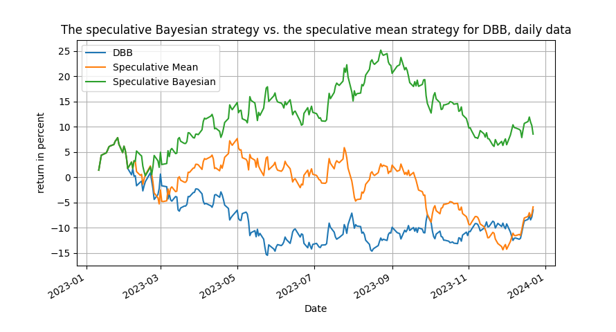
Figure 1: the speculative Bayesian strategy vs. the speculative mean and the passive benchmark, daily data for DBBta