By D. Thomakos
Creating trading strategies that have meaningful and interpretable economic foundations is crucial for both the understanding of financial markets but also for beating the "machine"! While it is true that a machine learning or artificial intelligence model can (possibly) uncover such relationships it is highly unlikely that the "machine" itself will give an interpretation or use it in decision making - I would be happy to hear your arguments if you disagree on this. Be that as it may, in this post I offer a very speculative strategy that is based exclusively on economic signals, similar to what we did in the last post but now with more variables and more foundations.
The idea has its origins in another early 1926 paper of the pioneer Holbrook Working titled "Bank Deposits as a Forecaster of the General Wholesale Price Level". The idea of Working, linking bank deposits with prices, recommends that deposits and producer prices must be linked with the financial markets: deposits are crucial for monetary liquidity and producer prices are crucial for the interplay of supply and demand. To this intuition I add something new and then bind things together: I add the relationship of retail sales with consumer prices, a natural economic pair that is linked with both demand and inflation. I form some new variables, see below, and then use them as trading signals with considerable success. First, let us see the input variables and then I will write down the signal variables and the trading strategy itself -- all data are from FRED. These are:
- Total deposits, all commercial banks, which are converted from the weekly to the monthly frequency; I shall denote this variable as [math]D_{t}[/math].
- The producer price index, for all commodities; I will denote this variable as [math]P_{t}^{p}[/math].
- The consumer price index, for all urban households, all items and US city average; I will denote this variable as [math]P_{t}^{c}[/math].
- Retail sales, of retail trade; I will denote this variable as [math]S_{t}[/math].
From these variables I construct my main signal variable as follows. I first take the ratio of deposits over the producer prices and also the ratio of sales to consumer prices, i.e., I define the variables [math] X_{t1} = D_{t}/P_{t}^{p}[/math] and [math]X_{t2} = S_{t}/P_{t}^{c}[/math]. I the take the monthly growth rate of all variables, the input variables and these two new variables -- all growth rates are denoted by smallcase letters. Then, I consider the following signal variables:
- [math] s_{t1} = x_{t1}-x_{t2}[/math] which has a number of different but meaningful interpretations. One can see this as the "real" deposits and sales (in the sense that are deflated by two price variables) or, alternatively, one can interpret them as the contrast between the difference of (deposits-sales) and (consumer inflation-producer inflation). When this variable rises we might think of it as an indicator of increased economic activity in a state of relatively low prices where there is potential for increased savings and investment opportunities.
- [math] s_{t2} = d_{t} - p_{t}^{c}[/math] which is the difference between deposit growth and consumer inflation; it has a similar interpretation as the first signal variable.
- [math] s_{t3} = d_{t}[/math] which is simply the deposit growth and used as a control in my experiments (to see if the information contained in the first two variables is essentially different from that of just deposits.
The trading strategies are both long/short and long-only and based on the delayed impact of the signal variables onto one monthly financial return, say [math]r_{tj}[/math] for assets [math]j=1, 2, \dots, M[/math], which we discuss below. Letting [math]\delta[/math] denote the delay of the signal variable I write:
[math] r_{t+1,j}^{h} = r_{t+1}\cdot sgn(s_{t-\delta, h})[/math]
[math]r_{t+1,j}^{h} = r_{t+1}\cdot I(s_{t-\delta, h} \geq 0)[/math]
for the long/short and the long-only strategies. As we will see in the results there is remarkable stability in the choice of "optimal" delay. Furthermore, and this is important for practical implementation, I find that the optimal delays in the backtesting are long enough in the past so that an investor can easily compute these strategies in real time!
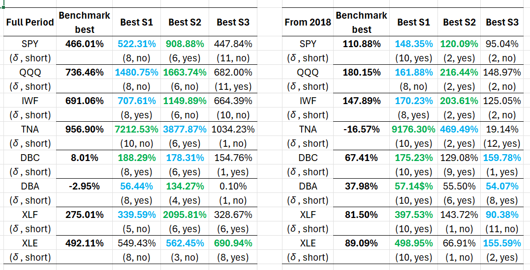
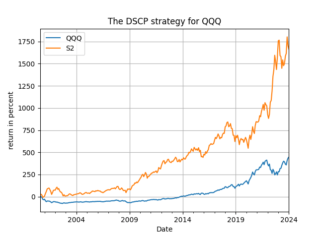
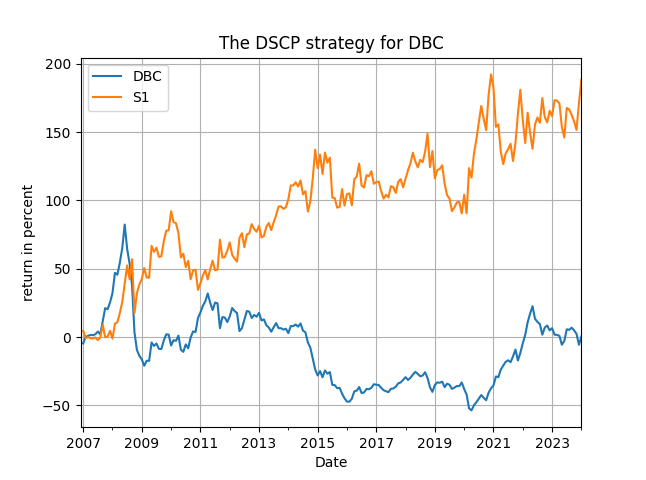
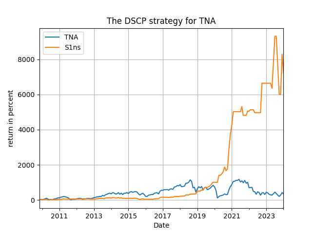
How do these signal variables perform in terms of their predictive power and trading performance? To examine this I am using monthly returns for several ETFs that we have seen in previous posts. These are: SPY, QQQ, IWF, TNA, DBC, DBA, XLF and XLE. Results are presented for the period post-2000 and then post-2018, with the maximum delay set to 12 months. I am using a direct search for the "optimal" delay but you can devise your own approach (do your research!) for getting close to optimal without this hindsight! The results appear below in Table 1, and some representative figures of total returns follow. Get the code from my github repository and then you can run additional experiments on the, speculative, efficiency of the method.
Table 1 has the results of my evaluation and they are, well, speculatively blasting! There is a number of significant findings in the table below which I outline immediately after it - keep reading!

Table 1. Results of the DSCP strategy, for the full period of available data and from 2018, monthly data
The first thing that you will notice is that the strategies based on the [math]s_{t1}[/math] and [math[s_{t2}[/math] signal variables are always outperforming (by a lot!) the passive benchmark. Thus, it is not just the deposits that drive these strategies but the combination of all the variables taken together. Second, you will see that for the three indices (SPY, QQQ and IWF) the best performing signal variable is the difference between deposit growth and consumer inflation, the [math] s_{t2}[/math] signal variable, either in the full evaluation period or the post-2018 period. Third, the application of the signal variables in the more "aggressive" ETFs (the leveraged TNA and the commodities and sectoral ETFs) is extraordinary and more, compared to the benchmark. In fact for the TNA the performance is making me wonder whether I made a mistake in the code but I think it holds true! Fourth, there is considerable, or more, robustness in the choice of the optimal delay across assets for each strategy with the most robust being the first based on the [math] s_{t1}[/math] signal variable: there the optimal delay's median value is 8 to 10 months (among the 16 cases examined in the table we have 7 times 8 months as optimal delay and 7 times 10 months). Finally, and I do not show the complete results here, both the long/short and long-only strategies usually outperform the benchmark.
A remark: this is a fully implementable set of strategies for real life practitioners, for the delays are such that data will always be available for making the computations. For the case when the delay is one month only (which is mostly for the last two strategies) one only has to revert to the first strategy that uses all four input variables where the delay is always greater than at least 5, and mostly 8, months.
These results are both highly practical and highly interpretable, the latter being a constant requirement if one has to tell a "story" as to why its strategy works. Here you have lots of things to discuss about the strategy's performance: the condition of the banking and the monetary system via the deposits, the state of supply via the producer inflation and the state of demand via retail sales and consumer inflation. Maybe you can come up with additional interpretations of the strategies or create your own early warning indicator about the state of the economy or the state of the market - that's homework and food for thought for another day, and in the meantime enjoy some speculatively good cumulative return plots!


