By D. Thomakos
Here is my pre-Christmas bonanza. This post was inspired by a comment by Giorgio Borelli in my previous post about the Osborne Bubble. Giorgio suggested to look at the fractional integration properties of the time series and consider including the estimation of the Hurst exponent, or order of fractional integration or long-memory coefficient, in my trading rule. In this short post I illustrate the estimation of this coefficient and I use it directly for trading. Results are very solid - which goes a long way to show that we should never let a comment unresearched!
The idea thus is very simple. In the representation of cumulative gross returns [math] x_{t} \doteq \prod_{j=1}^{t}(1+r_{j}) [/math], where [math]r_{j}[/math] are the period returns, given by the fractional difference below:
[math] (1-L)^{d}x_{t} = \eta_{t}[/math]
we want to estimate the long-memory parameter d, in the interval [0, 1] and then create a trading rule based on its magnitude. The rule works simply by shorting the market when we get into the area of non-stationarity (d > 1/2) and remaining long otherwise. Letting [math] \kappa [/math] denote a threshold for the long-memory estimate, the signaling variable becomes:
[math] s_{t+1|t} = I(\widehat{d}_{t} \leq \kappa) - I(\widehat{d}_{t} > \kappa) [/math]
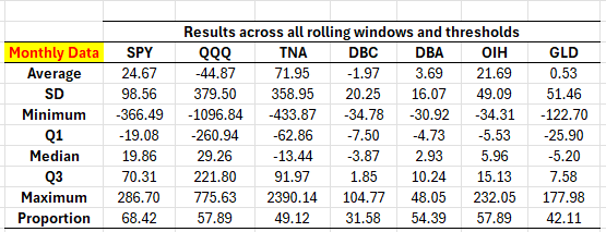
where [math] \widehat{d}_{t} [/math] is estimated by a rolling window of R observations before and including period t. I use Whittle's likelihood function for this estimation - code as always in my github repository. I have used the data from the previous post on the Osborne Bubble but at the monthly frequency, used a number of windows from 8 to 26 months (not a long enough sample for accurate estimation of the long-memory coefficient but the purpose is to allow trading) and three values of [math] \kappa \in \left\{0.5, 0.6, 0.7\right\}[/math]. I then aggregate the results across all parameter combinations and [math] \kappa [/math] threshold and report the corresponding statistics, for the total excess returns. The results appear in Table 1 below.

Table 1. Performance attribution of the fractional trader strategy. Monthly rebalancing, data starting in 2000, statistics are across all combinations of rolling windows and values of the [math]\kappa [/math] threshold, the delay is always 2-months, the range of rolling windows is 8 to 26 months, the table entries are in percent and correspond to total excess returns, proportion denotes the number of rolling windows that produced excess returns wrt to the benchmark. Please consult the Python code for more details.
The results are mixed, depending on the distributional measure one looks at. If we look at the average total excess return can see that is considerably positive only for SPY, TNA and OIH; if we look at the median total excess return then SPY, QQQ and TNA have it as considerably positive; if we look at the third quartile then it is positive for all assets: that is, at least 25% of the time across combinations the fractional trader strategy offered positive total excess returns. There is clearly a lot of volatility involved in this approach but one cannot but see that there is quite some promise in its use, particularly if the estimation of d becomes accurate or the threshold is chosen with some suitable, real-time, way. By the way, the results in Table 1 are for a delay of 2 months which makes the strategy easily applicable in real time.
But wait, there is more! Now, one can rightfully claim that the selection of the threshold [math]\kappa[/math] is not consistent with a real-life application, for it will require some cross-validation approach. While the claim is valid, we have a solution that appears to work well for the most volatile assets in Table 1: TNA, DBC, DBA and OIH. Here is the supercharger: we convert the trading rule to use as threshold the following running quantile of the estimated d:
[math] \kappa_{t} \doteq Q_{0.95}(\widehat{d}_{R+1},\widehat{d}_{R+2},\dots,\widehat{d}_{t}) [/math]
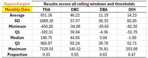
That is, we use as threshold the 95% quantile of the distribution of the estimated d up to time t - while keping the delay at 2 months, for a fully feasible strategy! The results are a blast, see Table 2 below.

Table 2. Performance attribution of the fractional trader strategy, supercharged. Details as in Table 1.
No comments are required! Don't wait then, go grab the Python code and experiment with the fractional trader strategy, supercharged! Merry Christmas!


