


By D. Thomakos
I frequently write about the importance of parsimony and simplicity in the context of quantitative trading strategies. Recognizing the importance of simplicity is critical for recognizing the value of complexity where is needed. Now here is the cue for this post: a 1936 article from the Journal of Experimental Education that defines the index of forecasting efficiency! In reality is a transformation of the correlation coefficient (although a non-linear one) and I give it trading flavor that works wonders!
First, let me set-up the problem I shall be addressing. Let [math] (y_{t}, x_{t-d})[/math] denote two assets, in the form of a dependent and explanatory variable with d being the delay parameter. The explanatory variable should be something more general, like an index or a commodity with wider impact on the market. If the explanatory variable leads the dependent, then one should be able to create a profitable strategy based on their relationship - and the index of forecasting efficiency works on that - like all proper correlations should. Before you dismiss the idea as too simplistic read-on - there is a catch to it!
The index of forecasting efficiency IFE is one minus the alienation coefficient i.e.,
[math]IFE_{t}(R,d) \doteq 1 - \sqrt{1-r_{xy}^{2}(R,d)}[/math]
where [math]r_{xy}^{2}(R,d)[/math] is the square of the sample correlation coefficient between [math] (y_{t}, x_{t-d})[/math] computed using a local window of R observations. The local window is not going to be large, as I have commented previously on my speculative correlation post (which you should check as well for that refers to a different correlation structure!). Now, how to you trade the IFE? Easy, here is how:
Step 1: Compute the IFE for several values of the delay parameter
Step 2: Find the value of [math]d^{*}_{\min} \doteq argmin_{d\in{\cal D}}IFE_{t}(R,d)[/math] that minimizes the correlation and also the corresponding value of [math] d^{*}_{\max}[/math] that maximizes it.
Step 3: Construct 4 trading rules based on either one of the above selected values of [math]d^{*}[/math] as follows.
Signal #1: trade using the sign of the correlation [math] r_{xy}(R, d^{*})[/math].
Signals #2, #3 and #4: trade using the sign of the explanatory variable at lags [math](x_{t-d^{*}-1},x_{t-d^{*}}, x_{t-d^{*}+1})[/math], with the latter lag being implemented only if [math]d^{*}\neq 1[/math] (else just follow the passive benchmark).
Signal #5: rotate between the 4 signals above by using the signal that has the highest NAV in the previous period (wealth rotation strategy).
That's it! The crucial choice in this idea is the variable used for [math] x_{t-d}[/math] and, as always, you can experiment with the choice of the local window R by getting your hands on the Python code available in my github repository. In the code you will find pair combinations of dependent and explanatory variables to see how and why the method works (yes, running the code will reveal which of the trading signals work and you should find the interpretation quite straightforward!). Here I will only illustrate the power of the suggested idea with two examples: one using the NASDAQ QQQ ETF and the stock of Apple (AAPL) and the other using the oil services OIH ETF and the gold GLD ETF - but it works in other pairs too! The results in the table below are for daily, weekly and monthly rebalancing: the daily rebalancing is for the period 2022-01-01 to 2024-01-31 and the weekly (for AAPL/QQQ) and monthly (for GLD/OIH) rebalancing is for the period 2019-01-01 to 2024-01-31. So, lets see the results below, in terms of total trading return.
Table 1: performance attribution of the efficient speculator strategy
The results, as you can easily see, are very supportive of the efficient speculator and, possibly more importantly, are supportive of the idea of simplicity against complexity - they also tally very with the previous post on the usefulness of correlation between returns and changes in returns. Of course you can experiment more with the Python code and find out more uses for this particular idea. Here is a hint: apply the efficient speculator methodology with [math]x_{t-d}[/math] being an economic variable and use monthly data. For example, how does inflation predict asset returns? If you want to see this, drop us a line!
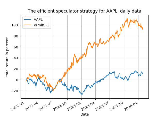
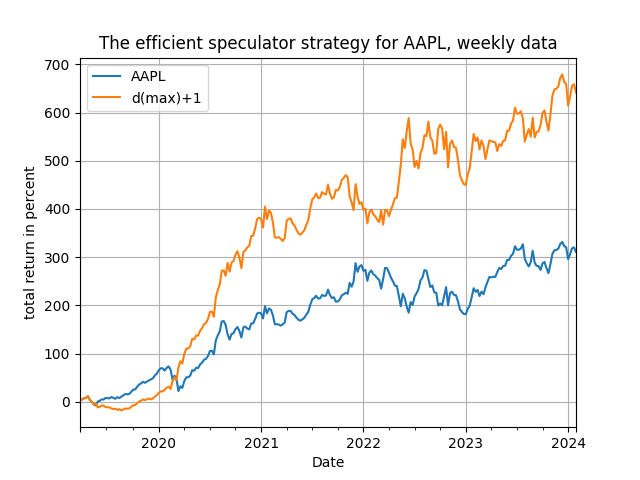
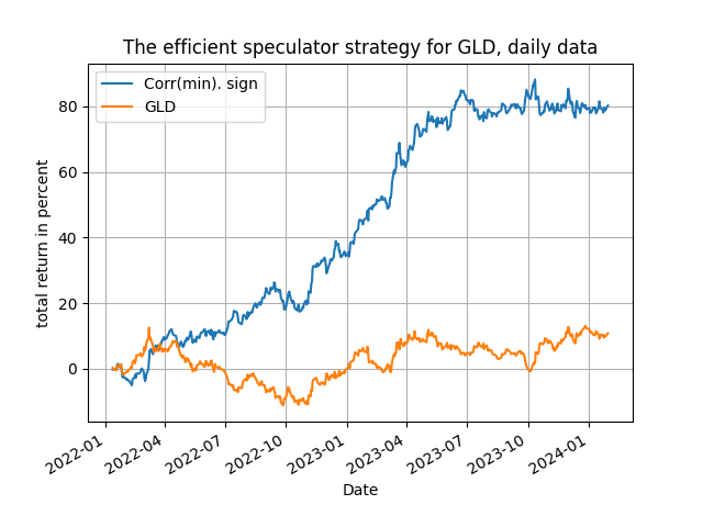
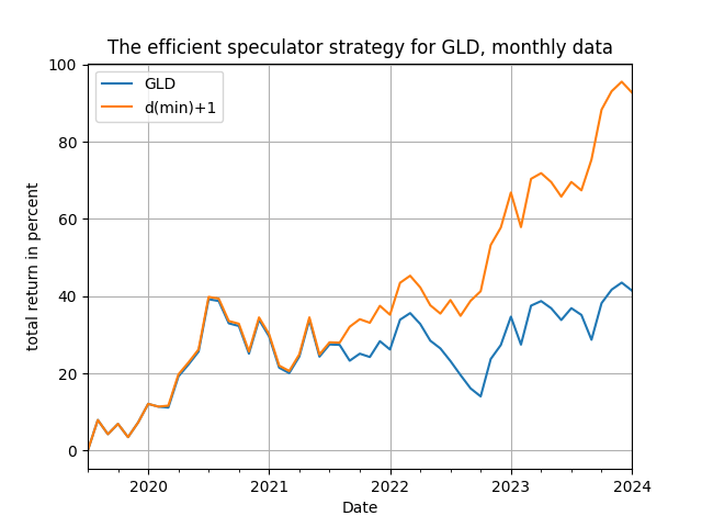
The four figures above show you the time evolution of the total trading returns of the efficient speculator strategy, for the same parametrizations as in Table 1 - and they are mighty satisfying! You will note that the frequency of the data and of rebalancing plays a role in the performance of the method, especially towards the end of the sample - but you can go and experiment a bit more and become yourself an efficient speculator!