By D. Thomakos
Happy New Year! This is our first technical post for 2024 and its going to be a follow-through of the last technical post here, on the use of the echo-state network (ESN) model. As promised then, in this post I will examine the efficacy of the ESN to generate profitable predictions - and what a great job that it does! What is very interesting, and you can explore it at depth in the Python code in my github repository, is that the ESN makes good predictions for financial returns using the Chebyshev basis polynomials - the implication being that market swings might be discoverable by this combination of the basis polynomials and the ESN.
I am using the same methodology as in my previous post, which I will outline below:
- Create the Chebyshev basis polynomials, that will be used as explanatory variables; note that since they will be applied to a stationary series (the returns) the degree could (should?) be higher than the one used for smoothing in the previous post.
- Select a sequence of dimensions for the state variable of the ESN; note that here the minimum dimension could (should?) be higher again than the one used for smoothing (this is natural since a trend can be less complex than a stationary series because it is dominated by its low frequency component).
- Select the frequency of training the network, the seed for the random elements of the state matrices and the number of initial observations to discard while training.
- Train the network by selecting the dimension of the state variable via the AIC.
- Use the trained network to predict the sign of next period's return, repeat and evaluate performance.
One nice feature of the ESN is that it does train easily for sign prediction, which is all that we want. Furthermore, all the results below were obtained with the same parametrization which suggests that the network is, potentially, quite robust to parameter selection. For my evaluation I will use daily data from the last six months of 2023 until today for several ETFs and the following parametrizations:
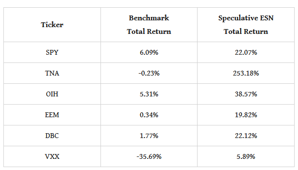
- an initial window of 21 days, a range of dimensions in the interval [14, 21], the random seed at 22, the leaking parameter at 50%, training the network every 5 days and a 4th order Chebyshev basis. That's it! Table 1 below has the results.

Table 1. performance attribution of the speculative ESN strategy vs. the passive benchmark, daily data, evaluation starts from July 2023
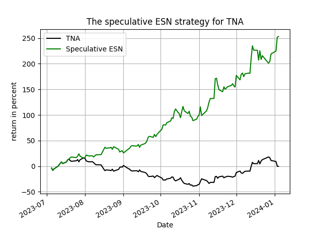
Not bad you say, right?! The performance is superb, especially for a period of time that has a large swing in the market. If you run the code to generate the figures for these ETFs you will also see that the ESN shoots-up very early on and stays well above the benchmark until the beginning of this year. The nicest plot is, of course(!), that of the TNA which I replicate below for your enjoyment - you would have been speculatively happy should you have known this model and used it this past summer!
There is a lot of things that one can learn by experimenting with this kind of network, such as for example the generation of complexity-weighted forecasts, as I did in this post on speculative complexity. In fact, the ESN is the ideal setting for doing just that because its output is defined by the dimension of the state variable that is the complexity factor of the network! I might be doing this in a follow-up post.

Figure 1. Figure 1: the speculative ESN strategy vs. the passive benchmark, TNA daily data, evaluation starts in July 2023, total return in percent


