By D. Thomakos
It is a frequent complaint that those outside the realm of speculation cannot use their skills for financial gain. Clearly this cannot be further from the truth, only if you know how to search and use these skills! Take for example climate change and rising temperatures - an issue of contemporary scientific and political significance: is it possible to use climate change for speculative purposes? In this post I show that it is. Not only the measured temperature anomalies can be linked to financial signals about future market positions but they can provide considerable excess returns, as I shall be illustrating. But be warned: there is more that meets the eye in the data I will be using and not all of the potential is revealed below. Do your own homework to find out what more you can extract from the material that follows!
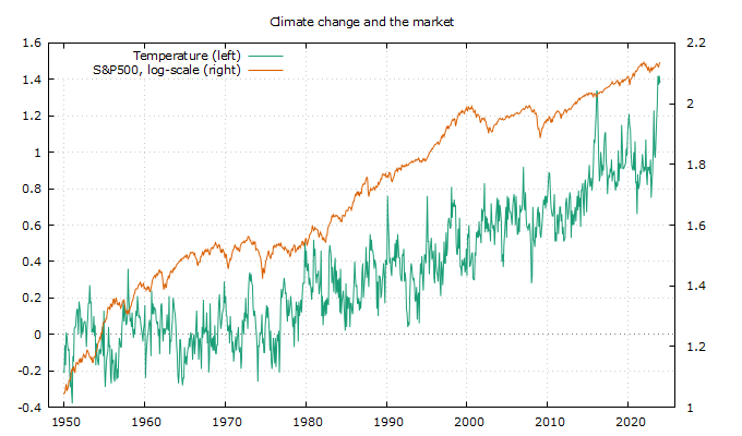
A speculative climatologist starts off with what he knows best, the data: you can get the time series of temperature anomalies at the National Centers for Environmental Information in a single click. I will use the most aggregative series, the one for land and ocean global temperature anomalies. The data are monthly and go a long way back, but we shall not be needing all of them. Then, I merge these data with the S&P500 monthly closing prices, crop them to start from 1950 and just hit the "make-me-a-strategy" button to roll some profits! Let's have a look at how the data look first in Figure 1 below.

Figure 1. Temperature anomalies, land and ocean globally, and the S&P500 from 1950
The data share the same trend, which is more pronounced over the long-term as in the picture. To get an idea of this common trend I estimate a simple regression on time and the results on the slope estimation are as follows (in pairs, with temperature first, all estimates are significant at the 1% level of significance): from 1950 (0.0012, 0.0011), from 1970 (0.0015, 0.0011), from 1990 (0.0018, 0.0008), from 2000 (0.0019, 0.0007) and from 2010 (0.0026, 0.011). Clearly temperatures have been rising faster than the market, on average, which means that their signaling capability should be time-varying - something that we will exploit to advantage. But before I get into the trading exercise, here is a quick look at one of the interesting regressions on the connection between the market and climate change, for the post-2010 period. I regress the log of the S&P500 on its first lag, time and a distributed lag of the temperature anomalies, followed by sequential model reduction. The result is an equation that is structurally stable and passes all specification tests, with the second lag of temperature being negative and significant and the ninth lag of temperature being positive and significant - however, their negative sum is not significant. The interpretation of this simple exercise is left for the reader - but the implications are rather clear: there is something out there. Let's find out more about it!
Since the temperature anomalies variable takes both positive and negative values, I can use it directly for signaling on my strategies, and I do this of course. In addition, I consider the change in the temperatures and the expanding (or recursive) mean of this change as three more signaling variables. Here are then my four variables on which trades of the S&P500 can be made, with [math] x_{t} [/math] denoting the original series of the temperature anomalies and [math] y_{t} [/math] denoting the monthly S&P500 return (a) [math] r_{t+1|t}^{1} \doteq y_{t+1}sgn(x_{t-d}) [/math], (b) [math] r_{t+1|t}^{2} \doteq y_{t+1}sgn\left(\sum_{j=0}^{t-d}x_{j}\right) [/math], (c) [math] r_{t+1|t}^{3} \doteq y_{t+1}sgn(\Delta x_{t-d}) [/math] and (d) [math] r_{t+1|t}^{4} \doteq y_{t+1}sgn\left(\sum_{j=0}^{t-d}\Delta x_{j}\right) [/math]. Once I do the recursive computations, I repeat them substituting 12-month rolling means in place of the recursive means above. Armed with these four signaling variables I then proceed to find the ex-post optimal values of the delay parameter d that maximizes total excess return [math]ER_{T}^{j}\doteq\Pi_{t=0}^{T-1} (1+r_{t+1|t}^{j}) - \Pi_{t=0}^{T-1}(1+y_{t+1})[/math]. I do this calculation from all years starting from 1950, 1960, 1970, 1980, 1990, 2000, 2005, 2010, 2015 and 2020. You can find all you need to replicate thins in my github repository, including the datafiles and a Gretl data file as well if you want to do the econometrics fast! I will only show results from 2000 because they are the only ones relevant in this discussion - and yes, you could have made lots and lots of profits if you followed this approach from, say, the 1970's. Go get the Python file and experiment to find out!

Table 1. Total excess returns from the use of the 4 signaling climate change variables, using a rolling and a recursive estimation for the mean of the change of temperature anomalies. In the (i, j) pairs we have the first element being the strategy or signal number as described in the text and the second element being the ex-post optimal delay d of the signal.
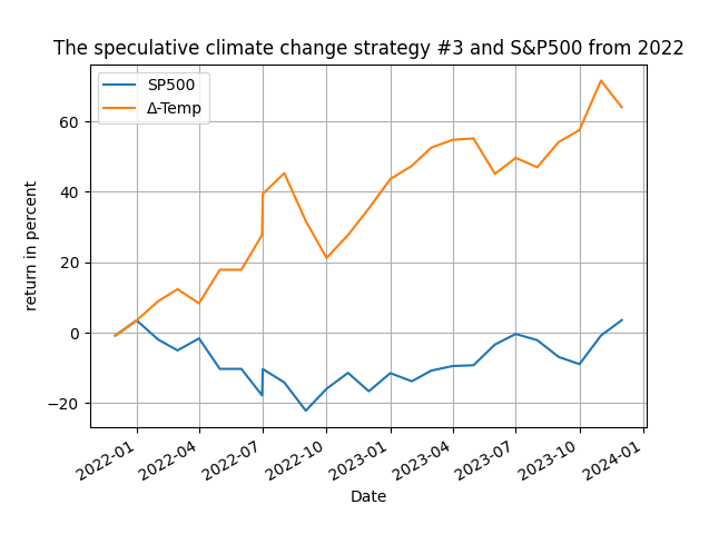
What's your conclusion from the above table? Would our climatologist be happy, speculatively happy, with these results?! Clearly the excess returns over the passive benchmark of the S%P500 justify the claim that there is some potential in generating speculative profits from climate change. However, as I noted in the introduction of this post, there is more to be learned and gained from these results - you should clearly exploit the association between the market and temperature anomalies in a more detailed fashion, maybe paying particular attention to the periods when the temperature dropped and not increased. Be that as it may, you could have made some very decent profits if you were to use the speculative climate change strategy and it would look on a figure too! Enjoy Figure 2 below and go experiment on your own on the impact of climate change in the markets!

Figure 2. The evolution of total returns for the speculative climate change strategy #3, monthly rebalancing


