By D. Thomakos
In recent past posts I explored the theme of echo-state networks (ESN) for smoothing, trend extraction and forecasting financial returns, and showed that this type of network has very good performance and potential as a method for addressing the above tasks. In this post I get into economic forecasting and the nuances of linear vs. non-linear models, the measurement of predictive accuracy and the time-varying ability of different models to capture the properties of economic time series.
I will focus on bivariate modeling, where [math]y_{t}[/math] would be the time series of interest and where [math]x_{t}[/math] would be some explanatory or "causal" variable. This is the simplest scenario for generating meaningful forecasts based on the evolution of one variable as connected with another and, yet, it is surprisingly powerful in applications - of course it is very easy to adapt this framework into one involving [math]\mathbf{x}_{t}[/math], a vector of explanatory variables - and you can do so by changing the Python code at my github repository! The generic form of the models I will consider nests in the following specification:
[math] y_{t} = f(\mathbf{z}_{t-d}, \mathbf{b}) + \epsilon_{t}[/math]
where [math]\mathbf{z}_{t-d}[/math] collects the explanatory variables (i.e., the lags of [math]y_{t}[/math] and [math]x_{t}[/math] but also the state variables in the ESN, and where [math]\mathbf{b}[/math] collects all the parameters. I consider four (4) forecasting models and one (1) forecast combination in the analysis that follows:
- if , and then the above general model collapses to naive benchmark.
- if , and then it collapses to the AR(1) benchmark (model AR(1)).
- If , and then it collapses to a linear transfer function with delay d (model LTF).
- If , and , where is the ESN state vector, then it collapses to a non-linear transfer function with delay d. Note that here $latex \mathbf{s}_{t}[/math] is a non-linear function of , built recursively (model ESN).
- I also consider a performance-based (past periods' cumulative MSE weights) combination of the forecasts from the AR(1) benchmark and the ESN forecast (model AR(1)+ESN).
All the above models have linear forecast functions and are very easy to compute. Yet, the ESN nests all of them and is more general and, therefore, amenable to additional analysis and model reduction. While I do not perform model reduction in this post it should be easy for anyone to do this and to select, with standard regression methods, which components of [math]\mathbf{z}_{t}[/math] to keep after training the ESN. Computing the forecasts is thus the easy part, but not the most interesting one! That is reserved for the experimentation with various parametrizations of the forecasting exercise and also for the evaluation of the forecasts across models. The series of the empirical illustration are all from the FRED database and are, in [math] (y_{t},x_{t})[/math] pairs:
Pair #1: advance retail sales (retail trade and food services) and CPI-based inflation
Pair #2: capacity utilization in manufacturing and advance retail sales
Pair #3: capacity utilization in manufacturing and industrial production in manufacturing
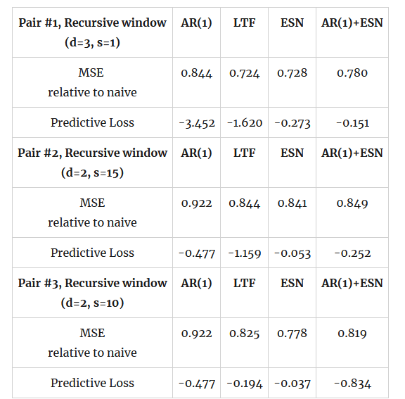
I estimate these models using both an expanding (recursive) window and a rolling window of 60 months and produce forecasts for one-month ahead, but report results on the recursive window only. The forecast evaluation is done with the standard measures such as the MSE and MAE but also with the coefficient of predictive precision and predictive loss that I used in this previous post. You can find the parametrizations used for the analysis in the tables below along with the results from the forecast evaluation - the initial date is 2000 and the evaluation starts 60 months later in 2005, going on until the end of 2023. Table 1 below has the results for the full sample evaluation and the "verdict" is clear: the coefficient of predictive loss is smallest uniformly for the ESN forecast, whose relative MSE is on par or smaller than the linear transfer function LTF. And not only that but note that the coefficient of predictive loss varies between the AR(1) model and the LTF model, although the LTF gives consistently smaller MSE. The ESN not only provides an overall better performance for its forecasts, but it also maintains its position as top performing model in most of the period of evaluation and captures better the large changes in the dependent variable.

Table 1. forecast evaluation of the three pairs, recursive estimation starting from 2006 and ending in 2023, d is the transfer delay and s is the dimension of the state variable in ESN
If the coefficient of predictive loss is a more robust measure of forecasting performance, and it better indicates forecast rankings, it might mean that we can use it to rank models based on their past performance and perform model and forecast rotation - and possibly do this in a better way than using past MSEs. I do this exercise of model and forecast rotation and the results are very encouraging. If [math]{\cal P}_{t-1,m}[/math] is the coefficient of predictive loss obtained from data up to and including period [math]t-1[/math], then I choose the forecast for period $latex t$ from the model that has minimum predictive loss (MPL), i.e.,
[math] \widehat{y}_{t|t-1}^{MPL} \doteq \left\{\widehat{y}_{t|t-1}^{m^{*}} : m^{*} = argmin_{m\in M}{\cal P}_{t-1,m}\right\}[/math]
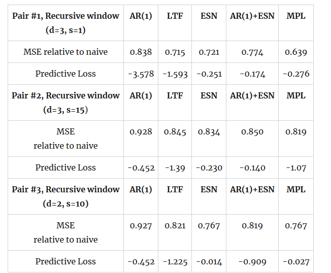
where is the set of the four forecasting models considered. Table 2 below has the results from this exercise where I estimated the predictive loss on an additional 60-month rolling window - this takes us into 5 more years into the evaluation period which now starts in 2010. The results are extremely suggestive for the potential of the coefficient of predictive loss, not only for forecast evaluation but also for model and variable selection. You will note in Table 2 that (a) using the forecast rotation we improve upon the individual models' MSE in all cases, (b) this occurs while maintaining a small (or smallest) coefficient of predictive loss and (c) if one was to choose for the potential explanatory variable in pairs #2 and #3 then the result would uniformly suggest that capacity utilization is better predicted by past industrial production rather than past retail sales.

Table 2. forecast evaluation of the three pairs, based on model and forecast selection using minimum predictive loss; evaluation starts from 2011 and ends in 2023; d is the transfer delay and s is the dimension of the state variable in ESN; the last column corresponds to the model that is selected by the minimum predictive loss of the previous period.
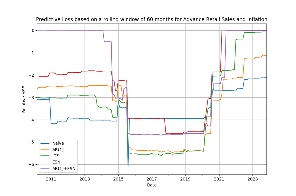
I illustrate the time-varying performance based on predictive loss for pair #1, the advance retail sales and inflation, in Figure 1 below. It is immediately apparent that there is scope for forecast rotation but, in this particular pair, this scope is limited as the ESN seems to dominate by having the smallest predictive loss overall, on average, and to performing particularly well after the Covid-19 crisis period (becomes more accurate faster and stays as a top performing model till the end of the evaluation period).

Figure 1. time-varying estimation of the coefficient of predictive loss for pair #1, rolling window of 60 months
Here are some key takeaways from the above analysis:
a) the ESN is a robust model for forecasting, as it includes both a linear and a non-linear component and nests an LTF model with the same explanatory variables.
b) the ESN is robust in the choice between rolling and recursive estimation window; it performs uniformly well with an expanding window thus eliminating the need for rolling window selection - this is in contrast with the LTF (or the AR(1)) model which might perform better with a rolling window (which one?!)
c) Standard measures of predictive accuracy such as the MSE or the MAE do not necessarily coincide in their model rankings with the measures of predictive loss and, importantly, the use of minimum predictive loss can assist in model and forecast rotation for improving most or all performance metrics.
d) static, full-sample, measures of predictive accuracy are not as informative as time-varying ones and one would gain additional information about model robustness and model performance if he or she looks at the static and dynamic measures at the same time.
Grab the Python code from my repository and experiment for yourselves. The code is easy to understand and easy to "cannibalize" for your own projects. Discover the forecasting power of the ESN and the robustness of performance evaluation based on the coefficient of predictive loss - you can also work more on the model selection approach for the dimension of the state variable in the ESN as in previous posts thus adding one more layer of automation in your code!


