By D. Thomakos
Accurate measurement of economic activity is an important aspect of data collection in every economy and the real GDP is by far the most popular and comprehensive measure of this activity that we currently have available. But monitoring, collecting and updating data on real GDP is neither easy nor straightforward and is subject to revisions - plus a GDP measure can be computed from either the demand or the supply side of the economy and is forced to obey various income identities. In this post I illustrate that the cyclical properties of real GDP can be easily, conveniently and immediately captured by a much simpler measure - that is fully interpretable! I will first define and discuss this new measure and then will examine its cyclical properties to illustrate that it almost perfectly matches to the cyclical properties of the real GDP.
In previous posts, see here and here, I have made use of the capacity utilization measure in manufacturing, which correlates inversely with unemployment and can be used as a predictor of economic activity and the financial markets in many contexts. Let then [math] X_{t1} [/math] denote the quarterly capacity utilization in manufacturing (as percent of total productive capacity) and let [math] X_{t2} [/math] denote the quarterly mortgage debt service payments as percentage of disposable personal income and define a third variable as their difference, i.e., define [math] X_{t} \doteq X_{t1}-X_{t2}[/math] and then take first differences to obtain [math] x_{t} \doteq \Delta X_{t} [/math]. Finally, compute the quarterly growth rate of quarterly real GDP and denote it by [math]y_{t}[/math]. The claim made is that the temporal and cyclical properties of these two variables are essentially identical!
To explore this claim I take the available data and compute (a) the plain correlation of the data [math]\mathbb{Corr}(y_{t},x_{t})[/math], (b) the correlation between the spectral densities [math]\mathbb{Corr}(\hat{f}_{y},\hat{f}_{x})[/math], (c) the average squared coherence [math]\bar{S}_{yx}[/math] across the whole frequency spectrum, (d) the correlation between the autocorrelation functions [math] \mathbb{Corr}(\hat{\rho}_{y},\hat{\rho}_{x})[/math] and, finally, (e) a normality test and a sign test for the difference of the series [math]z_{t} \doteq y_{t}-x_{t}[/math]. All these measures are computed for the full available sample and many subsamples, and the results demonstrate a remarkable consistency. Note that the use of the properties of the [math] z_{t} [/math] series implies that we are testing for some form of randomness; if the two series share the same cyclical characteristics, then their difference should be essentially white noise. Even so, I use the [math] z_{t} [/math] variable as a trading signal - with considerable success. I consider the trading strategy that uses a lag of this variable to trade the S&P500 using the rule:
[math] r_{t|t-1}^{Z} \doteq r_{t} \cdot sgn(z_{t-d}) [/math]
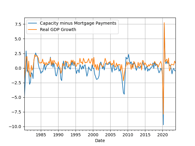
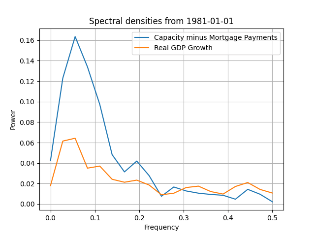
with [math] r_{t} [/math] being the quarterly return of S&P500 and with d = 2 being the optimal delay (this incidentally makes the Z-strategy fully implementable in real-time!). So, let's take a look at the data. I first start with a plot of the data, in Figure 1, and you can immediately see the correspondence of the two series. Their scales are very close to one another, even if I put them into different axes, their cycles are almost the same and have similar volatility (the full-sample standard deviation of the series is 1.46 for [math] x_{t} [/math] and 1.10 for [math]y_{t}[/math]). In Figure 2 I have the estimated spectra for the full-sample, and you can also see there that, beyond the power difference, the shape of the spectral densities is basically the same.

Figure 1. The quarterly change of capacity utilization in manufacturing minus mortgage payments and the quarterly growth rate of real GDP

Figure 2. The full-sample spectral densities of the quarterly change of capacity utilization minus mortgage payments in manufacturing and the growth rate of real GDP
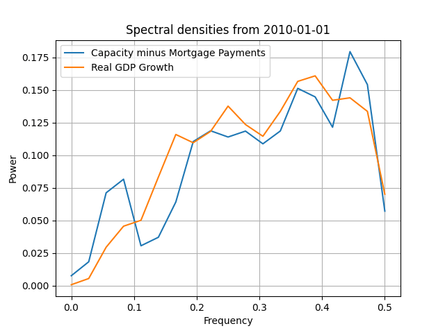
In Table 1 below I present all the statistics mentioned before for many different time periods, plus the total excess return of the z-strategy over the passive benchmark of the S&P500. The claim made earlier, that this new series of capacity utilization minus the mortgage payments is a very good proxy for real GDP growth, seems to be consistently validated. The data correlations are over 80% and the become increasingly higher as we move to 2019: from 81.54% in 1981 to 96.13% in 2019. The correlations of the spectral densities are also very high but more erratic, as they start higher for the full-sample and stay the same or become small as we move the sample forwards. There is a "break" starting in 2000 and then 20o5, where this type of correlation gets small or vanishes entirely - we will see the change that occurs in the spectral densities later on. That the two series are strongly correlated can be seen also from the column of the average squared coherence, where we see that progressively it becomes larger as we move after 2000 and especially after 2010 and 2015. In Figure 3 you can see the new shape of the spectral densities after 2010 (which remains the same for 2015 and 2019); you can spot the difference between Figure 3 and Figure 1 easily, for the former shows increasing power at higher frequencies indicating a "tighter" connection between the two series (and a reduction in the space of variables that affect the real GDP growth). This spectral shape might be an effect of the large swing of growth because of the Covid-19 pandemic but this is what the data are telling us. The next column in Table 1 has the correlation between the autocorrelation functions of the two series and there we can also see that they are consistently higher than 90% implying the same memory structure for real GDP growth and our new variable.
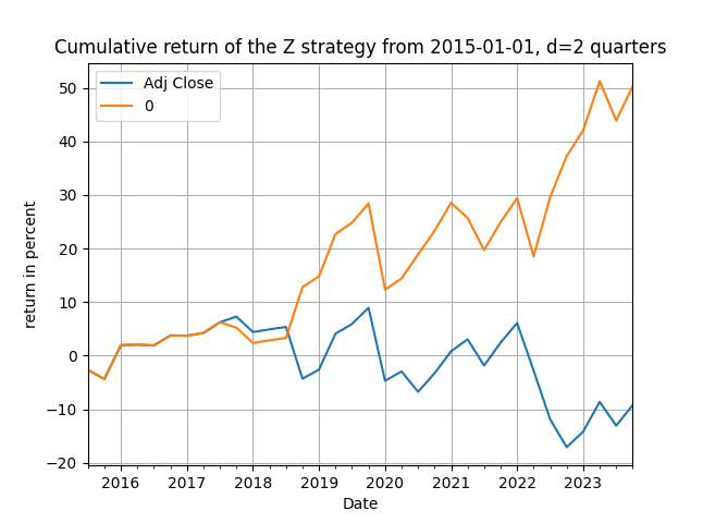
Turning next to the last three columns we can say even more about the properties that related the two series. The [math]z_{t}[/math] variable of the difference between growth and capacity utilization minus mortgage payments is normally distributed with p-values over 10% everywhere and the sign test for randomness also has p-values that are higher than 35% everywhere across subsamples. These results reinforce the similarity of the characteristics between the two series and validate the previous ones above. What's left is the last column that has the total excess return [math] ER \doteq \prod_{t=0}^{T}(r_{t|t-1}^{Z}+1) - \prod_{t=0}^{T}(r_{t}+1)[/math] of the strategy against the S&P500 benchmark. The results are telling for two reasons. First, you can clearly see that there is informational content in the z-strategy: when the Z-variable is rising implies a heating of the economy (the GDP has many other components besides manufacturing after all) and recommends buying the market - and the reverse when its falling. Second, the performance suggests that although the Z-variable passes the tests of normality and randomness, as a abstract random variable, nevertheless has information that relates clearly to market direction. Figure 4 has the evolution of total return from 2015 onwards, and you should note that it is after the spectral break of 2005, and especially after 2015, that the two series are very much aligned - this justifies the performance of the Z-strategy.

Table 1. Statistics on the similarity between the quarterly change in manufacturing minus mortgage payments and the quarterly growth rate of real GDP, see main text for column definitions
The fast-paced modern economy has some particular aspects that are worth further study. As noted above, the dimension of the space of useful economic information might be much smaller than was in the past - this is what the results of this post suggest, with just two variables capturing the magnitude and cyclical aspects of the (more complicated) real GDP growth. Be that as it may, you can get the Python code from my github repository and experiment for research or for speculation - for all our posts have both flavors with a preference for speculative investment returns!

Figure 3. The spectral densities of the quarterly change of capacity utilization minus mortgage payments in manufacturing and the growth rate of real GDP, from 2010

Figure 4. Cumulative returns of the S&P500 passive benchmark and the Z-strategy, quarterly data


