


By D. Thomakos
Paying tribute and acknowledging the contributions of the past is an important part of promoting our scientific and social understanding. In this post I thus consider building a "barometer", the name that was most frequently used in the beginning of the 20th century to describe economic and financial indices used to represent, track and forecast the business cycle! A very representative example is that of a 1916 American Economic Review paper by Warren M. Persons "Construction of a Business Barometer Based on Annual Data " - but the references are many from that era!
The approach I follow has these steps (all data are the for the US downloadable from FRED, please see the Python file in my github repository):
1. I first construct two indices based on monthly data. These are called [math] I_{t1}[/math] and [math] I_{t2}[/math], described below, and then are combined into a single index by plain averaging, i.e., [math] I_{t3} = 1/2 \cdot (I_{t1}+I_{t2})[/math].
2. I convert the monthly indices to quarterly by downsampling, averaging across the three months of each quarter.
3. I then use the thus created "barometer" to examine its cross-correlation properties vis-a-vis the real GDP growth.
4. Finally, I go back to my monthly indices and use them to trade the economic cycle based on the S&P500.
You should consult the Python file for the details, but here are the important highlights on what is going on! For the [math] I_{t1}[/math] index I use 3 components: the ratio of the personal consumption expenditures to the CPI, the ratio of total consumer credit to total bank credit and the ratio of business loans to total bank credit. The index is the average of these three variables. For the [math] I_{t2}[/math] index I use a single component: the difference between the unemployment rate and the 10-to-2 year spread of US treasuries - this index turns out to be very very useful and, importantly, it does not coincide with the characteristics of unemployment and (as we shall see later on) provides good trading signals. Figure 1 below has the final index [math] I_{t3}[/math] after downsampling to quarterly frequency:
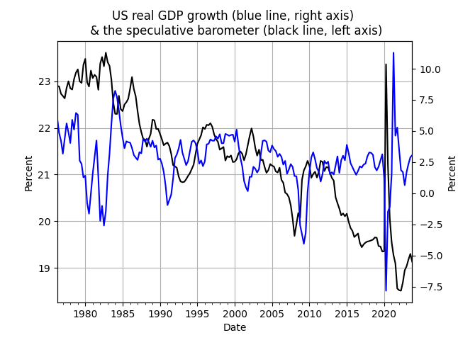
Figure 1. the speculative barometer index and the US real GDP growth, quarterly data
It should be easy to see the leading indicator properties of this new index [math] I_{t3}[/math], our speculative barometer! The strength of this index is particularly evident across the whole period of examination. Performing the cross-correlation analysis, I find that the speculative barometer has essentially zero contemporaneous correlation with real GDP growth (an important characteristic of any leading indicator!) and reaches is maximum positive correlation at a lag of 4 quarters (one year). Although I have not performed a forecasting exercise to examine the usefulness of the barometer in predicting real GDP growth (which is a nice idea for a term or research paper!), a natural question that arises is this: can we use the speculative barometer as constructed to predict market movements? Is it, as we would like to find out, truly speculative?!
For this part I take the monthly values of the barometer and build a few trading strategies that appear to work very well, particularly after 2000 and onwards. I did my backtesting with the S&P500 but you can substitute any financial asset and repeat the analysis - very easy and, trust me on this, very profitable for certain asset classes! I describe my main strategy below and more details in the Python code.
My main signaling variable is [math] s_{j}\cdot sgn(I_{t-k,j})[/math], where [math] s_{j}[/math] is a sign-changing variable depending on which index is being used, and [math] k[/math] is the delay of issuing the signal for trading. I have [math] (s_{1}=1, k=4)[/math] and [math] (s_{2}=s_{3}=-1, k=2)[/math], and the economic interpretation should be obvious for the sign-changing variable! I also consider another signaling variable that combines the above as [math] sgn\left[s_{1}\cdot sgn(I_{t-4,1})\right] + sgn\left[s_{2}\cdot sgn(I_{t-2,2})\right][/math]. Table 1 below has the performance characteristics of these speculative barometer strategies, evaluated after and including 2008:

Table 1. performance attribution of the speculative barometer strategies, monthly data, evaluation starts from 2008
The speculative barometer does indeed work, well, speculatively! You can easily spot the outperformance compared to the passive benchmark, both in terms of total return and in terms of lower maximum drawdown. Furthermore, and this is important, you will note the dramatic fall in maximum drawdown for the strategy that combines the signs of the two component indices of the barometer, without sacrificing (too much that is!) total return. Figures 2 and 3 that follow have the evolution of the cumulative returns of these strategies and also the annual total return by year.
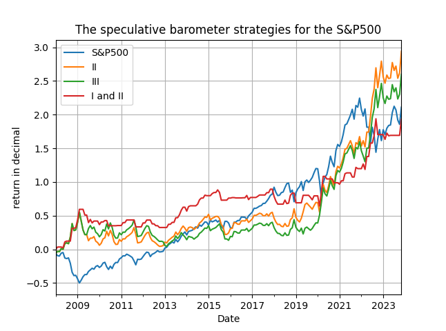
Figure 2. cumulative returns of the speculative barometer strategies and S&P500, monthly data from 2008
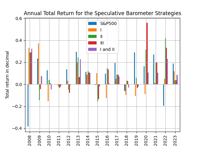
Figure 3. annual total returns of the speculative barometer strategies and S&P500, monthly data, by year, starting in 2008
Have a careful look at these figures and find out what is the secret ingredient for the performance of the speculative barometer strategy and where should be using it in your economic and financial monitoring. History is a guide to new research ideas and financial secrets to be exploited!