By D. Thomakos
Learning is a concept that I have highlighted in many previous posts and is still fascinating. In this post I illustrate another method that learns from past forecasting errors; the method is similar in spirit, but not in method and interpreration, to that of adaptive learning. It works with any forecasting method as its input and its parameter-free, the only choices to be made are those of two rolling windows. For my empirical examples I will be using both continuous and discrete data, explained below, and as an input forecasting method the sample mean.
Consider thus the continuous returns [math] r_{t} [/math] and their signs [math] s_{t}\doteq sgn(r_{t})[/math]; I shall use [math] x_{t} [/math] to denote either of the two types of data. Let [math] x_{t+1|t}(R) \doteq R^{-1}\sum_{j=t-R+1}^{t}x_{j}[/math] denote the input forecast, as the plain sample mean of a rolling window of R observations. After a period of some initial observations start updating the input forecast with the following formula:
[math] y_{t+1|t}(R, B) \doteq x_{t+1|t}(R) - b_{t|t-1}(B)[/math]
where [math] b_{t|t-1}(B)\doteq B^{-1}\sum_{j=t-B+1}^{t}\left(x_{j} - y_{j|j-1}\right)[/math] is the estimated bias of the "learning" forecast and where B is a second rolling window.
In contrast to adaptive learning, where the input forecast is adjusted by the learning parameter and the last forecast error, here learning takes place exclusively from the use of the bias - and do note the negative sign (do the math to understand its importance! it makes sense). The only selections here are those of the rolling window pairs (R, B) - in the empirical implementation below I just use the ex-post optimal values from a range of choices for these two windows. In real practice one can use any method that cross-validates such choices - check past posts about this problem of ex-ante choice of windows and how to solve it.
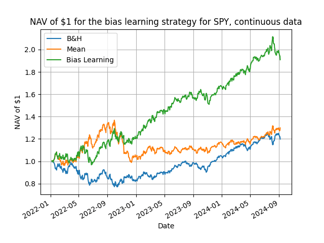
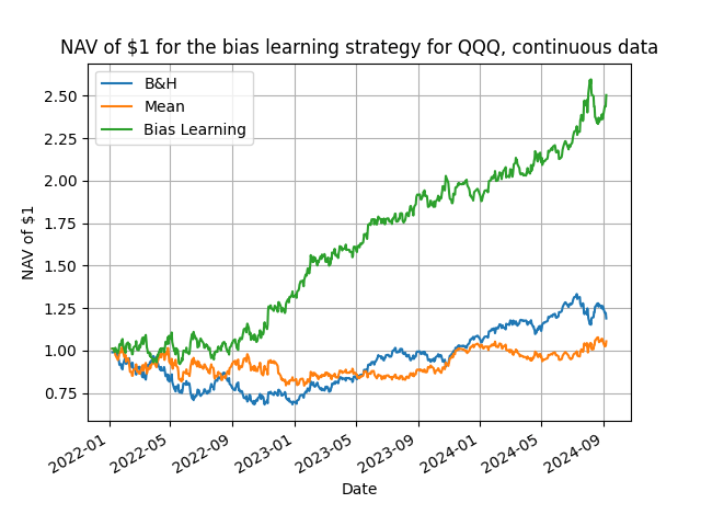
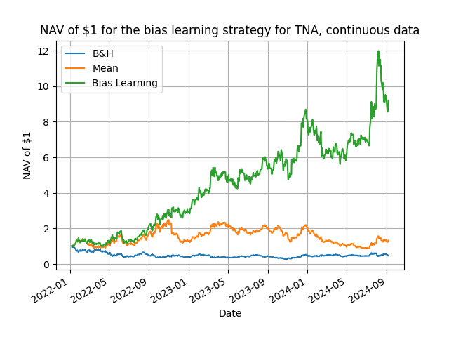
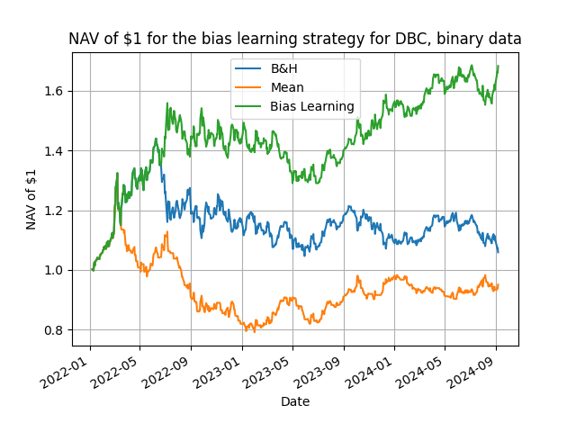
That's all there is to it, and does the method work you ask? You bet it does! Below I present some representative results from daily rebalancing using a variety of ETFs plus the Bitcoin and Ethereum, starting from 2022. In the Python code in my github repository you can make changes and experiment with different trading frequencies and assets.
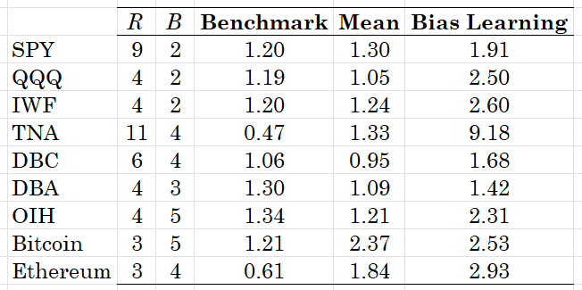
Table 1. NAV of $1 for the speculative bias learning strategy. The benchmark is the buy & hold passive strategy, mean is the sample mean forecast strategy and bias learning is the speculative bias learning strategy explained in the text. The best ex-post parameter combinations are shown. Daily rebalancing with the data starting in 2022.
The results validate, one more time, that learning is feasible and profitable. Points to note are three: first, the relatively small values for the B rolling window over which one computes the bias learning (makes sense, you will only consider your more recent forecast errors); second, for 6 out of the 9 assets considered we have that R > B; third, the outperformance of the bias learning strategy is quite considerable with a median, over these assets, excess return of 109% over the mean input forecast and of 131% over the passive benchmark. These are numbers not easily dismissable on their speculative value!
As I have argued many times in the past, essentially in all posts, simplicity rules supreme when it comes to financial forecasting. I would wonder how more complex models would do and what sort of outperformance one should obtain from complexity. Enjoy the plots below and make sure that you always benchmark your strategies in the motto "novus ordo speculationis simplicitatis et parsimonia est".
