By D. Thomakos
The interplay between renting and buying residential property is an important real estate, economic indicator that relates with core variables such as inflation and economic growth, as well as monetary policy and interest rates (that in turn determine mortage rates that are of importance to home buyers and renters alike). In this post I explore the relative prices of rent inflation vs. housing prices inflation and find that they have leading indicator properties for a segment of the market. That this is so is not an unreasonable proposition: higher relative prices of rents vs. housing prices possibly imply a rising valuation of homes (since the present value of rents should be an indicator of future housing values) and a rising real estate market is always good for the economy and the financial markets. I thus gather some data from FRED, on the value of houses [math] x_{t1} [/math] and on the rent of primary residence [math] x_{t2} [/math] - both series are indices and at the montly frequency. I take their ratio and then the growth rate of the ratio to constuct my leading indicator as in [math] x_{t} \doteq \Delta \log(x_{t2}/x_{t1})[/math]. I link my explanatory variable via two simple regression models, with my dependent variable say [math] y_{t} [/math] which will be the monthly return of one of several ETFs that I will consider in what follows.
The forecasting models are very basic, trivial one would say. Nevertheless they work wonders and are highly interpretable when used for trading. Thus, consider the model:
[math] y_{t} = \alpha + \beta x_{t-d} + \gamma I(x_{t-d} \leq 0) + \epsilon_{t} [/math]
which has the drift variable [math] I(x_{t-d} \leq 0) [/math] and where d is the delay of the impact of the leading indicator into the market returns. When I set [math] \gamma = 0[/math] and the drift term is not there I denote the model as "Rent & Buy #1" and when I allow [math] \gamma \neq 0[/math] I denote the model as "Rent & Buy #2". Some positive delay, maybe greater than one month, is required because the transmission effects from the real estate property market to the financial market might not be immediate. Once the model is estimated, and I use both ordinary least squares and robust reqression, the forecasts are immediate to obtain, [math] \widehat{y}_{t+1|t} \doteq \widehat{\alpha} + \widehat{\beta}x_{t-d+1} + \widehat{\gamma} I(x_{t-d+1} \leq 0) [/math], as are the trading signals, as follows:
[math] \widehat{y}_{t+1|t}^{RB} \doteq y_{t+1}\cdot I(\widehat{y}_{t+t|t} \geq 0) [/math]
You will note that, unlike many or most of my previous post, the trading signals here are long-only. This is of course the result of experimentation but it does have an economic explanation. The signal variable need not necessarily indicate a market reversal when the forecast becomes negative, but it does signify a robust economy when positive - for the reasons we discussed earlier.
The data for the dependent variable are montly returns for the ETF proxy of the S&P500, SPY, and three sectoral ETFs from the index, namely financials XLF, energy XLE and technology XLK. You can of course experiment with any ETF of your choice by getting your hands in the Python code in my github repository. The table below summarises optimal perfomance for each of these ETFs, for the maximum available history of each, starting from 2000. You can easily experiment with other starting dates and parameter combinations. All results below based on robust estimation, save for the XLK ETF that uses ordinary least squares.

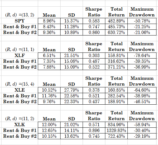
Table 1. Results of the Rent & Buy Strategy vs. the Passive Benchmark, monthly data from 2000 or later depending on availability
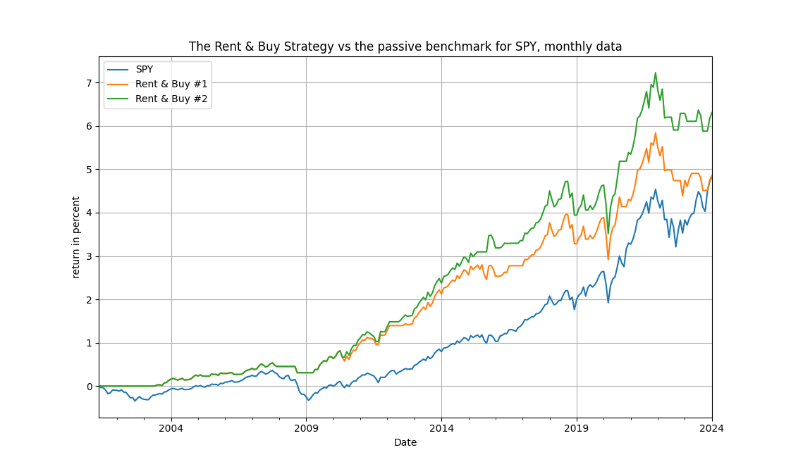
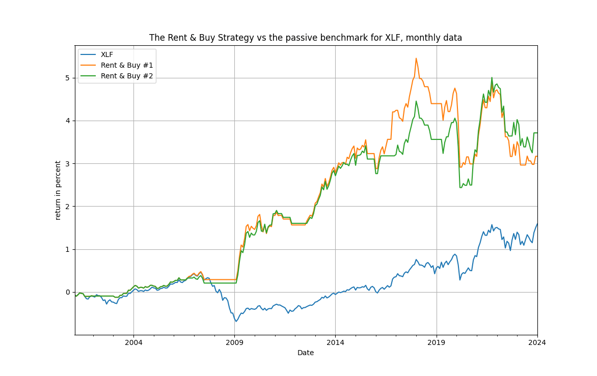
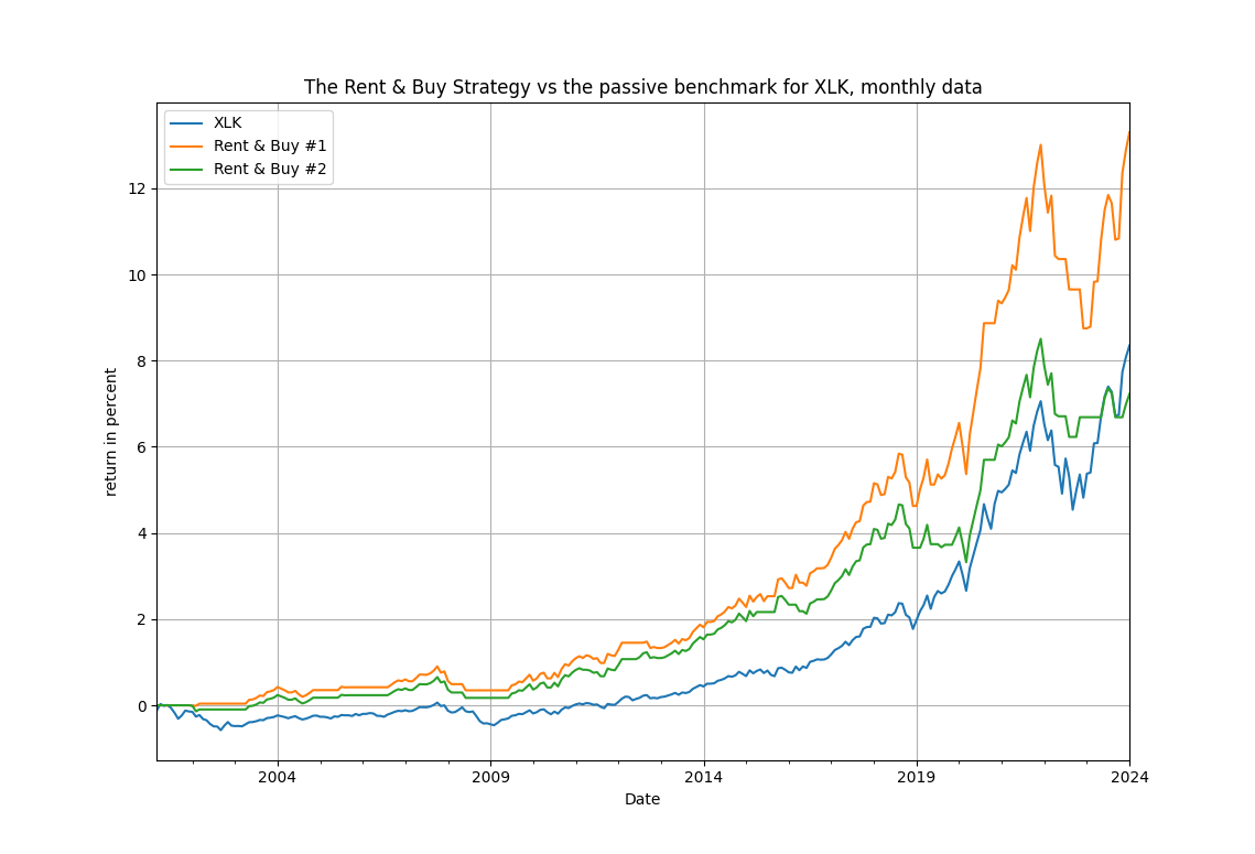
Three results are immediate by looking at Table 1. First, the signal variable works very well by providing not only excess returns but also considerably lower maximum drawdowns and higher Sharpe ratios. For example if you consider SPY you will see an excess return of over 150% and more than half the maximum drawdown of the index itself. Similar results can be see for the other ETFs in the table. Second, note that for the energy and technology ETFs the simpler model works way better than the more complicated with the drift term. Third, the lower maximum drawdowns that are observed suggest that the strategy will possibly be out-of-the-market in critical downturns. The figures below actually bear that as essentially true.
The cumulative returns rise steadily and fast, obviously with the volatility of their underlying benchmark, but note they avoid the large drops (save for the Covid-19 period) and remain consistently above the benchmark. Also of note, in the second figure below, is that for the financials the exit timing from the 2008 financial crisis is almost perfect. All in all, the rent-to-housing prices ratio works as a trading indicator, makes economic sense, is easy to apply and it's only up to you to experiment more in different asset classes. Rent or buy, let the profits run high!


