

")
By D. Thomakos
Consider the constant forecast function [math] x_{t+1|t} = \alpha_{0} [/math] and augment it with a simple rule of error learning as in [math] x_{t+1|t} = \alpha_{0} + \alpha_{1}^{+}I(e_{t|t-1} > 0) + \alpha_{1}^{-}I(e_{t|t-1} \leq 0) [/math]. Using the properties of the indicator function we may also write [math] x_{t+1|t} = (\alpha_{0} + \alpha_{1}^{-1}) + (\alpha_{1}^{+} - \alpha_{1}^{-})I(e_{t|t-1} > 0)[/math]. Condensing the initial parameters, we can then write:
[math] x_{t+1|t} \doteq \beta_{0} + \beta_{1}I_{t|t-1}^{+} [/math]
where I define [math] I_{t|t-1}^{+} \doteq I(e_{t|t-1} > 0)[/math]. Examining the forecast error we find that is equal to [math] e_{t+1|t} = (x_{t+1} - \beta_{0}) - \beta_{1}I_{t|t-1}^{+}[/math]. Taking expectations on both sides we find that the expected forecast error is equal to [math] \mathbb{E}(e_{t+1|t}) = (\mathbb{E}(x_{t+1}) - \beta_{0}) - \beta_{1}\mathbb{E}(I_{t|t-1}^{+})[/math]. Assuming (local) stationarity we have that an unbiased forecast requires that [math] \beta_{0} \doteq \mathbb{E}(x_{t+1}) = \mu[/math] and an adjustment for the probability of a positive forecast error [math] \mathbb{P}(e_{t|t-1} > 0) \doteq \mathbb{P}_{t| t-1}^{+}[/math]. We can then write the form of the unbiased forecast function as follows:
[math] x_{t+1|t} = \mu + \beta_{1}(I_{t|t-1}^{+} - \mathbb{P}_{t|t-1}^{+}) [/math]
It is now immediate to see that the forecast is going to be the mean of the time series and it will be be adjusted to the direction of the last forecast error compared to the existing expectation of positive forecast errors: if the last forecast error was positive a positive adjustment will be effected (raise the forecast); if, on the other hand, the last forecast error is negative then a negative adjustment will be effected (lower the forecast). When raising the forecast the magnitude depends on one minus the rate of positive errors and when lowering the forecast the magnitude depends on minus the rate of positive errors - and both these magnitudes are scaled by [math] \beta_{1} [/math] which, as we shall now show, has to be positive to minimize the mean-squared error (MSE) of the forecast.
Let us then compute the MSE explicitly to find what the value of [math] \beta_{1} [/math] should be. Computing the new forecast error we find it to be [math] e_{t+1|t} = \left(x_{t+1} - \mu\right) - \beta_{1}(I_{t|t-1}^{+} - \mathbb{P}_{t|t-1}^{+})[/math], from which we can easily compute the MSE as in: [math] \mathbb{E}(e_{t+1|t}^{2}) = \mathbb{E}(x_{t+1}-\mu)^{2} + \beta_{1}^{2}\mathbb{E}(I_{t|t-1}^{+} - \mathbb{P}_{t|t-1}^{+})^{2} - 2\beta_{1}\mathbb{E}(x_{t+1}-\mu)(I_{t|t-1} - \mathbb{P}_{t|t-1}^{+}) [/math]. We can immediately see that the MSE of the forecast will be smaller than that of the sample mean (i.e., smaller than the variance of the time series) iff the following conditions hold (a) the covariance between the time series and the series of positive forecast errors has to be positive and (b) the parameter [math] \beta_{1} [/math] has to be positive and to obey: [math] \beta_{1} \leq \mathbb{E}(x_{t+1}-\mu)(I_{t|t-1}^{+} - \mathbb{P}_{t|t-1}^{+}) / \mathbb{E}(I_{t|t-1}^{+} - \mathbb{P}_{t|t-1}^{+})^{2}[/math] with strict inequality probably preferable; clearly, if the covariance between the time series and the series of forecast errors is negative then then parameter [math] \beta_{1} [/math] has to be negative as well to maintain our argument of MSE reduction. In this latter case the inequality changes direction and we should have that the parameter [math] \beta_{1} > 0[/math] and in particular [math] \beta_{1} \geq \mathbb{E}(x_{t+1}-\mu)(I_{t|t-1}^{+} - \mathbb{P}_{t|t-1}^{+}) / \mathbb{E}(I_{t|t-1}^{+} - \mathbb{P}_{t|t-1}^{+})^{2}[/math]. Note that in either case of a positive or a negative covariance we will end up estimating the absolute value of the parameter, that is [math] \vert\beta_{1}\vert[/math].
If these conditions hold then we should be able to forecast better, a priori, than the sample mean. However, the fact that an inequality is required implies that estimating [math] \vert \beta_{1} \vert [/math] is not sufficient. We shall need an inflating/deflating factor, let's call it [math]\gamma [/math], which will force the forecast to use either a smaller or a larger value than [math] \vert \beta_{1}\vert [/math]. I experimented with the following specification that appears to work quite well: [math] \gamma \sim \lambda \log(t) [/math], where [math] \lambda \in \left[0, 1\right] [/math], for deflating [math]\beta_{1} [/math] and where [math] \gamma \sim \lambda^{-1} \log(t) [/math] for inflating [math]\beta_{1} [/math]. The final forecast function is now written as:
[math] x_{t+1|t} = \mu + \gamma \vert \beta_{1} \vert (I_{t|t-1}^{+} - \mathbb{P}_{t|t-1}^{+}) [/math]
which is what I shall be using in my application. It should be clear from the structure of this forecast function that it cannot be applied to data that are (locally) trending and thus they offer infrequent sign changes; it is much better suited to series that have frequent sign changes: yes, this means financial returns but also economic series that appear in first and not in seasonal differences. An example would be monthly vs annual inflation: the monthly inflation exhibits more frequent sign changes than the more trending annual one. For the empirical illustration I shall be using the following series obtained from the FRED database and, as usual, the Python code can be found in my github repository. The results below are/should be self-explanatory but read the caption to the Table!
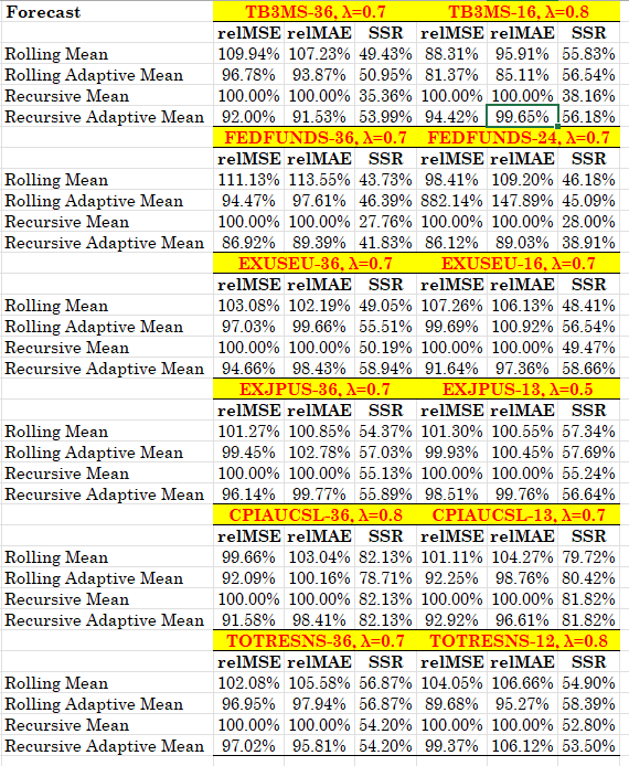
Table 1. Relative forecasting performance of the adaptive mean forecast function, the benchmark being the recursive mean. The FRED ticker is given along with the rolling window and the parameter λ. relMSE is the MSE relative to the benchmark, relMAE is the MAE relative to the benchmark and SSR is the sign success ratio (the probability of a correct sign prediction). All data are monthly starting from 2000. All series are in their monthly growth rates, except the interest rates where they are given as monthly differences.
The results are very much supportive to the use of this new forecast function and you will see that it works across a range of different economic variables. Furthermore, there is very reasonable stability (almost uniformity) in the choice of the λ parameter which implies that possibly little work needs to be done in selecting it. There you have it, starting from the constant forecast function, adding error learning, de-biasing and then regressing (but with an MSE minimizing twist!) you get your adaptive mean forecast. Enjoy and, I would rather recommend, use it as a very comfortable forecasting benchmark.