


By D. Karaoulanis
1. INTRODUCTION
Nonlinear dynamics is a branch of mathematics, which has experienced a very large growth in the last 60 years, mainly due to the increasing computational power of computers. The emergence of nonlinear behavior in many dynamical systems describing natural systems, revealed the chaotic character with which nature manifests itself. Although the equations describing such systems are relatively simple, the behavior of such systems is complex and sometimes very difficult to predict.
The dependence of the evolution of a system on the value of a system parameter indicates the sensitivity to change of such a system. Concepts such as attractors, limit cycles in Phase Space and various techniques such as Lyapunov exponents are tools that help to understand and predict the evolution of such systems. However, the stochastic behavior observed in particular systems highlights the difficulty of predicting and determining the factors that determine that particular behavior. When it comes to safe prediction, that's what it's all about.
The study and development of a set of time series is one of the key issues of concern in the field of Economics. The problem of forecasting the evolution of such a time series is essential, especially in the financial markets. The occurrence of a chaotic behavior in a time series (even if the factors that influence it are known) raises the question of whether and to what extent one can predict and to what extent. The mathematical tools of nonlinear dynamics may offer a measure of description of the system under study, but a safe prediction is in many cases a problem to solve.
In this article, we will refer to chaotic time series, showing simply and understandable the methods and tools used to study them. We believe that it will be seen that there is a possibility of predicting their evolution, if the factors affecting them are known. Our hope is that this article, with its summary mentions, will be an incentive for someone to investigate further the topic, which is one of the most interesting and promising in the field of Economics. After all, who wouldn't want to know how a stock will develop, whether or not to invest in it?
2. NON-LINEAR DYNAMICS-CHAOS
Each of us remembers from his school years, or from the first year of university, the course of introduction to Newton's Physics, and especially in regard to the part called classical mechanics. We had been taught Newton's three laws, which direct and describe the evolution of a physical system. We were greatly impressed by the fact of the deterministic character of the description, giving us the feeling that our understanding of nature and its changes was fully comprehensible and explicable. Especially, the statement that the knowledge of the initial conditions of the system, and the use of the laws which describe it, lead to a full prediction of its evolution. We felt that man had already understood the mechanisms of nature's functioning and could apply them absolutely with the aim of scientific progress and the improvement of his daily life. The technological achievements we have experienced as humanity in our daily lives have more than validated this belief. Even the hard-to-understand Theory of Relativity validated this determinism.
However, in the early 20th century, the emergence and subsequent consolidation of quantum mechanics, to describe the microcosm, shifted the question of prediction from the certainty of Newtonian mechanics to the possibility only of knowing the probability of the occurrence of a particular event. Quantum theory and its results upset our view of safely predicting the evolution of a physical system and of the values of the variables that describe it. However, this dispute was about the microcosm and its interactions and not about phenomena involving the macrocosm that could be predicted with sufficient accuracy.
However, this belief that the phenomena of the world we live in and understand with our senses had found their full description based on the laws of classical mechanics came to be challenged by a great mathematician, Henri Poincare, in the late 19th century posed the so-called problem of three bodies, interacting with each other by Newton's gravitational force (the problem remains unsolved to this day). He showed that the orbit of a body which receives the gravitational interaction of two or more other bodies cannot be predicted. Poincare was the first to formulate the possibility of chaotic evolution in a gravitational system of three and more bodies, demonstrating that small causes can cause substantial changes in the behavior of the system. So he introduced chaos into the Solar System.
It took more than 80 years for astronomers and others in different fields to realize the importance of this discovery. Scientists around the world began to realize that several nonlinear dynamical systems could not be given a single prediction for their evolution. Of decisive importance and contribution was the discovery made by another scientist, meteorologist Edward Lorenz, and concerned the study and evolution of phenomena occurring in the Earth's atmosphere. The model of the atmosphere he was working on consisted of a system of nonlinear differential equations. The solutions of the equations he took were different and sensitive to the values of the variables included in his equations. He concluded that the forecast of any weather conditions depended essentially on the values of the model parameters. Lorenz's results led to the famous phrase: "A butterfly flying in Hong Kong can cause a storm in New York."
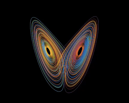
Figure 1. The Lorenz Attractor.
The emergence of chaotic behaviors in various systems under study in various scientific fields alarmed scientists. Here lay hidden a great truth about nature, which had to be thoroughly investigated. Chaotic behavior was discovered in Medicine, Biology, Chemistry, Economics, and the list kept growing. In recent years chaos theory has occupied musicians, psychoanalysts as well as writers. The inability to predict accurately has puzzled scientists whether we finally know the laws that describe nature and whether the tools we have will ever be able to give us some final answers to the questions we are asking. The principle of cause and expected effect has now been called into question, and it is now necessary to investigate the factors which bring this principle to a crisis.
But now let's look at what a dynamic system is what its main characteristics are and what are the possibilities for its solution. A dynamical system is defined as any system of interacting physical, chemical, and biological variables that evolve over time according to specific laws. The only independent variable is time, which can be either continuous or distinct. A dynamic system of continuous time it requires for its study the solution of ordinary differential equations, while a dynamical system of discrete time is described by difference equations. The fact that their independent variable being discrete means that we do not observe them constantly, but at regular intervals.
Linear differential equations, like linear dynamical systems, are quite easy to solve. On the contrary, the case of nonlinear differential equations and nonlinear systems is quite difficult to solve. Why nonlinear systems are so difficult to analyze compared to linear ones? Τhe essential difference is that linear systems can be analyzed in parts. Then each part can be solved separately and finally by combining the individual solutions we have the total answer. This idea allows for an imaginary simplification of complex problems, and is found in methods such as in normal oscillation modes, Laplace transformations, at the beginning of superposition and Fourier analysis. In this regard, a linear system is exactly equal to the sum of its parts.
But many natural systems don't act that way. Whenever the parts of a system interfere, or cooperate, or compete, nonlinear interactions occur. Most systems from everyday life are nonlinear, and the principle of addition fails spectacularly. As mentioned above, such physical systems are described by a system of differential equations, the solutions of which describe the time evolution of the system. Since these differential equations are nonlinear, an analytical solution of them is often impossible. For this reason, scientists use alternative methods of solving (numerical methods) to visualize the solutions for these systems. One such mathematical illustration of the dynamical system is the so called phase space. Having the representation of the phase space, we can predict the future evolution of the system. Different initial conditions (input values) or different values in the parameters that affect the system, can lead to different trajectories of evolution in the Phase Space.
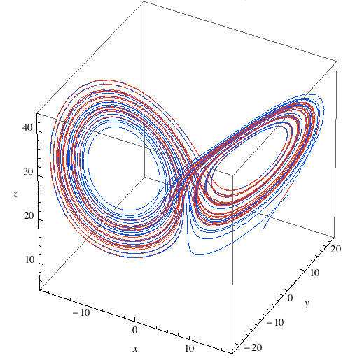
Figure 2. A Phase Portrait for a dynamical system
Another element that contributes substantially to the prediction and evolution of the state of the system is the so-called equilibrium points. They are the points of the phase space where the instantaneous change of its description variables is equal to zero. These points are characterized as stable or unstable depending on the future development of the system when it finds itself in this state. A stable point is a point at which, when the system is found, an imposed minor disturbance (a slight change in initial conditions) cannot remove it from that state. In contrast, when the system finds itself in an unstable place, then a small disturbance removes it from it, sometimes drastically. Finally, there are the cases where the system can be found in the so-called limit cycle, which indicates that the system is going through a process of periodic repetition of its behavior. A point is declared to be totally stable if the system returns to it, regardless of any initial conditions.
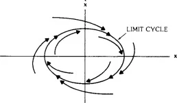
Figure 3. The limit cycle case for a dynamical system
A typical example of a chaotic system whose evolution prediction is impossible to make is weather. Based on existing Weather description models, for an accurate forecast of weather conditions, accurate knowledge of temperature and atmospheric pressure values is needed, values that enter into the initial conditions of the description model. However, since measuring instruments have a limited accuracy of a few decimal places and it is necessary to know these values at every point in the atmosphere (which is impossible), any prediction is achieved within the framework of average values and approximate predictions. For such a system, where the distances of the regions examined are large, it is expected that deviations from the predicted behavior will sometimes be large, revealing the properties of a chaotic attractor.
In concluding this brief reference to the chaotic behavior as it manifests itself in various physical systems, as well as the characteristics of this behavior, we would like to emphasize the fact that the lack of predictability in these kinds of systems is not due to an incomplete knowledge of the laws and equations that describe them. It is the differential equations and the parameters within them that determine such behavior. The nonlinearity of these equations as well as the interdependence of the parameters makes the time evolution of these systems in the long run unpredictable. However, the mentioned mathematical tools help substantially to understand this behavior in combination with as accurate knowledge as possible of the values of the parameters that affect these systems.
The main reasons that make it difficult to use these mathematical tools to safely predict the evolution of such systems, could be said to be the following:
・Few and no representative data sets.
・These methods work more precisely in the case where no noise appears in our data. Simulations of such systems using a computer, in many cases, ignore the existence of noise in the data, which obviously does not exist in real conditions.
・These methods were developed and applied to systems of few dimensions and work quite satisfactorily in them. However, for multi-dimensional systems, determining chaotic behavior is much more difficult, making it difficult to predict the time evolution of the system.
・The introduction of appropriate parameters concerning the system under study may also be questionable. The use of the exact model to describe the system is an essential condition for its observed (real) evolution.
For all the above reasons, dealing with such systems requires great care both in the selection of the appropriate model and the parameters involved in it and in the correct use of mathematical tools for a safe and error-free drawing of the necessary conclusions.
3. CHAOTIC TIME SERIES
A very interesting structure shown in Phase portraits is one related to the concept introduced into dynamical systems as an attractor. What is an attractor? An attractor for a dynamical system that manifests chaotic behavior is a point or set of points in the Phase Space, toward which such a system tends and from which it cannot escape as time passes. Indeed, in the case of strange attractors (such as the Lorenz Attractor), strange orbits appear in the space of the phases in which the system remains, without escape. One could therefore speak of a kind of steady state that can be found in the system, where a set of points of the Phase Space appears periodically. If the attractor is chaotic, then it is highly sensitive to initial conditions, however the state trajectories observed are confined within the limits of the attractor. Thus, a dynamic system characterized by a chaotic Attractor is locally unstable but completely stable since the system never moves away from the attractor Basin. It is obvious that in the case of a chaotic attractor, although the system is characterized by a degree of stability, it is nevertheless impossible to accurately predict the future state of the system when the initial conditions change even a little. In this case the displayed trajectories may show a large deviation, precluding predictability. Starting from a specific point (initial state of the system) in the phase space, it seems impossible to predict which trajectory within the boundaries of the attractor the evolution of the system will follow.
AIn this part of our analysis, we will focus on studying the time evolution of a time series and whether such a data series can manifest chaotic behavior and to what extent. We will therefore deal with the dynamic evolution of the process or system that produces the magnitude we observe and therefore we will consider that we observe the magnitude in time with a fixed time step, i.e. with a fixed sampling time. A set of such observations is called a time series. In some problems the sampling time may not be constant and then more specific processing of the time series is needed to perform the analysis. For example, the daily prices of the stock market constitute a time series with variable physical sampling time.
However, the sampling time of the measurements of the time series must remain constant if we want to draw safe conclusions about the various variables that affect it. If some measurements are further apart than the sampling time, the corresponding empty spaces may be filled by an interpolation method. It shall also be checked whether any data received has values that are much greater or less than the overall set of measurements, which may be due to errors in the measuring instruments or caused by the way in which they were obtained. Another issue concerns the amount of data that should be measured in combination with the time frame within which it was measured. Fewer points than are necessary is almost certain that will lead to erroneous conclusions.
The main characteristics to be studied for time series, before adapting a model that describes the evolution of it, are stagnation, trend, periodicity, determinism or stochasticity and of course linearity or non-linearity of it.
By stagnation, we mean to see whether or not the observed variations in time series values vary with time. In the case of a non-stationary time series, certain trends may occur, i.e. slow changes in its mean values over time, which should be checked. Also, in the case of a non-stationary time series, its values may display a periodicity, which may refer to specific time periods (per month, per quarter), they are also called seasonal. Such behaviors are important and should be included in our analysis, as they are important determinants of the evolution and predictability of the time series.
All the time series, which refer to real-world data, contain noise and in this sense can be characterized as stochastic. Any analysis of such data should therefore focus on investigating and identifying the deterministic part that directs the time series. When the cause of the evolution of its values is not clear due probably to noise and generally does not seem that this cause dominates its evolution, then the particular system is characterized as stochastic and only conclusions derived from a purely statistical study can be drawn. Again, if for some reason, we can assume that there is a deeper cause justifying the behavior of the system under study accompanied by some stochastic fluctuations, but not dominant in the evolution of the system, then we can apply some techniques involving deterministic dynamical systems, such as locating main periods if the system seems to exhibit a periodicity, or techniques for nonlinear potentials exhibiting a chaotic behavior.
Finally, the occurrence of linearity or non-linearity in such a system seems to be directly related to the deterministic or non-deterministic evolution of such a system. By the term linearity we define that all variables of the system can be expressed as linear combinations with respect to the parameters of the system. This means that for a linear system, the future evolution of the time series can be expressed as a linear combination of its previous observations, which cannot be true for a nonlinear system. In a nonlinear system, the nonlinear interaction between the parameters requires additional data based on the previous observations. Especially in the case of a linear deterministic system, with no noise, the analysis is relatively simple, giving solutions easily determinable (fixed point of convergence, periodic points or trajectories). In contrast, in the case of a nonlinear dynamical stochastic system, it is quite difficult to identify nonlinear dynamical relationships so that conclusions about the evolution of that system are quite precarious.
In order to be able to determine the chaotic nature of a time series and in addition to predict its evolution, the following conditions are necessary:
・The system under study should have a small number of variables (a system of few dimensions). As pointed out above, in chaotic systems where the number of variables is large, the usual mathematical techniques do not give reliable results so that the system is considered random and not chaotically deterministic.
・We should have a large number of observations (thousands) with a small amount of noise. Theoretically, we should have an infinite number of measurements, but this is obviously impossible. Small multitudes of measurements cannot give safe data of system behavior, not allowing an accurate description model to be derived.
・Also, an important factor is increased accuracy in observations, with as many decimal places as possible. The current computational power of computers allows processing such data accuracy by simultaneously extracting numerical results of the same accuracy.
・Finally, the time series should exhibit behavior of increased stagnation without long-term trends. What is desirable is for the series to keep its statistical properties (average, variance) relatively constant over whatever period of time we study it.
In classical statistical time series analysis linear features of the series such as mean values, dispersion and the so-called autocorrelation coefficient are studied. The study of the dynamic system is done using linear models such as ARMA (auto regulatory integrated moving average model), models which give satisfactory results in the case of linear processes but do not satisfactorily describe nonlinear processes. Applying linear analysis to the case of real time series with stochastic nonlinear features, much of the information is lost and received as noise. However, this piece of information can refer to a deterministic nonlinear behavior and can only be studied and retrieved using nonlinear methods of analysis. Of particular interest are nonlinear dynamic systems of small dimensions (with a small number of variables), such as pseudo-periodic systems and chaotic systems.
The dynamical systems that describe a chaotic time series are energy loss systems, i.e. systems where the initial "volume" of values of the system's variables in the Phase Space constantly shrinks. Each trajectory of evolution of these systems is attracted towards some invariant set of points, which is the attractor of the system. When studying such a chaotic time series, the nonlinear features of the system are sought, e.g. the dimension of the attractor of the system and its degree of complexity. These features are defined, based on the theory of nonlinear systems, as invariant measures of the system, which do not change over time as well as by the observation process.
For the analysis of a chaotic time series through the tools of nonlinear dynamics, the basic prerequisite is the reconstruction of the phase space of the system, without altering its characteristics, but its shape is not preserved during the reconstruction process. The theorem that provides the necessary conditions, under which we can have a smooth reconstruction of the observed Attractor, is the Takens theorem. What Takens demonstrated is that it is possible to derive the relationship between the dynamical behavior of the system and the observed variables, without necessarily knowing anything about the system under study. This can be done through the time delay method, which allows the construction of several time series of the system, using only the original time series. With this conversion, a variable of the system is converted into a series of variables of shorter time length, which however provide for each time a point in the new space that has been created. The method of time delays provides the possibility of extracting the "hidden" information found within the data of the time series. However, an incorrect choice of delay time and the dimension of the newly reconstructed phase space combined with the existence of extrinsic noise in the system can lead to incorrect conclusions about the evolution of the time series. Empirically, the choice of delay time should be such that it is the least possible integer where discernible changes are observed in the observed data. As for the new dimension of the phase space, it should be chosen so that the observed attractor retains its topological characteristics in the new space.
There are many classes of nonlinear models for describing a chaotic time series. These models are divided, according to how they are defined in the state space, into universal, semi-local, and local.
・Universal models have unique analytic expression for the entire domain of definition. Such models are polynomial and fractional.
・Semi-local models are analytically expressed like universal models but they consist of a set of basic functions, and for this their form changes in the different regions of the state space. Such models are neural networks and radial basis functions.
・Local models do not have unique analytic expression for the whole domain but are configured differently in each region of the state space. Such models are kernel models and local linear models.
These dominant types of models, although applied to the description of the evolution of a chaotic time series, sometimes give reliable results while in other cases they require improvement and adaptation by introducing parameters that substantially affect the system. The nonlinear behavior of data requires very careful application if we want a reliable though approximate forecasting. We would like to stress again that if the system is chaotic, then it is sensitive to initial conditions and therefore whatever is the suitability of the chosen model, the predictability is limited to a short time horizon, thus increasing uncertainty in forecasting its evolution.
Because the problem of predicting the evolution of a time series is the main purpose of analyzing them, the most prevalent prediction models are local models. In these, the analysis focuses on the part of the reconstructed space of the time series that we are interested in making the prediction. In this way, even if the entire series manifests a chaotic character, the trajectories that manifest in this limited space, that we are considering slowly and gradually evolve, allows us to make a short-term prediction. These models, strange as this may seem, have been widely accepted in the field of forecasting and have been improved in recent years by methods of optimizing the parameters that influence the future development of the system. It examined how to reconstruct the phase space that would not change the topological features of the original space and how the prediction time depth could be extended and what are the main factors determining this depth.
The issue of noise in the data is an important factor that should be taken into account. Noise affects the form of the reconstructed space, and therefore the proximity of the points we are considering. In local forecasting, in combination with a small number of adjacent points, it can be the main reason for failure in the forecast estimate, because in addition to the intrinsic indeterminacy of the reference point, the nearest neighbors will also have indeterminacy, which could not be adjacent points if the reconstruction was done without noise. For a better and more reliable forecast, a larger number of adjacent points should be taken. Another question that arises concerns the sampling time window and the process of reconstructing the Phase Space. If we increase the time window, will we achieve a better forecast? Is there an optimal reconstruction or a specific time window, with which we can achieve very good prediction regardless of the future time depth we want to predict? As shown by the study of such systems using local models, there is no such possibility of combination. It was observed that if we increase the time window no better predictions are achieved, rather the opposite.
Specifically, for the case of chaotic but deterministic time series, the models used to study and predict their evolution are based on the assumption that there is a stable relationship between the predictor variable (dependent variable) and certain parameters (independent variables) that affect it. This relationship can well be described as a cause-and-effect relationship. In these models, the existence of independent parameters, offer the researcher the possibility of finding many scenarios of evolution of the system with the ultimate goal of finding the optimal scenario. However, these models have serious drawbacks, such as needing a large amount of information about both the variables of the system and the parameters displayed in it. Finally, there are many cases where the production of complete forecasts from such a model requires previously estimating, on the basis of some other forecasting method, the future value of certain input variables.
Concluding this section on chaotic time series and the models that attempt to describe their behavior, we would like to comment on the criteria that determine the choice of optimal prediction. The main criterion for choosing a forecast method is the time horizon, i.e. the length of time to which the forecast will refer in the future. Qualitative methods are generally used for long-term forecasts, while quantitative methods are used for medium-and short-term forecasts. Also important is the number of periods for which provision is required. Some techniques are suitable for predictions corresponding to one or two periods after the most recent observation, while others to more. There are also techniques that combine prediction horizons with different lengths of time. Another important factor is the cost of a prediction method, which is determined by the amount of data required by the method and the complexity of its implementation. In many cases where choosing the appropriate forecasting method is not easy, it has proved preferable to combine the forecasts resulting from the application of different methods. This increases the accuracy of forecasts as the interval of variation of errors is significantly reduced.
In many cases where the choice of the appropriate forecasting method it is not easy, it has proved preferable to combine the predictions resulting from the application of different methods. This increases the accuracy of forecasts as the interval is significantly reduced variation of errors. Assuming stability of data behavior patterns, the optimal theoretical model would have to produce the most accurate predictions. But once these patterns change in practice, combining predictions from different models produces an average that is closer to reality than the theoretically more correct model. Using a combination of predictions is tantamount to assuming that it is impossible to find a model that optimally determines the behavior of historical data. But the study of the various techniques of combining predictions can ultimately lead to the identification of more appropriate patterns of behavior and therefore to the creation of better individual models. If the combination of different models produces more accurate predictions, it is theoretically possible to construct a model that makes optimal use of the different forms of information contained in the predictions of those models.
4. CONCLUSIONS
In recent years, much emphasis has been placed on finding methods of extracting information from a range of data, such as time series. The discovery of some patterns in the behavior of these data led to the development of some methods and tools with the central goal of predicting the evolution of such systems. In particular, for the case of time data displaying chaotic behavior, the tools developed for the study of nonlinear dynamical systems were used. It is not a lack of knowledge of the laws or equations that describe the behavior, but about the intrinsic property of nonlinear dynamical systems to exhibit sensitivity to the initial conditions as well as to the values of the parameters that direct the system. Despite their deterministic simplicity, over time these systems can produce completely unpredictable and Divergent (or chaotic) behaviors.
The main reasons that cause practical difficulties in using these tools in real data are the following:
・Small or unrepresentative samples of time series data.
・The existence of noise in the data. Study methods work best with clear and accurate data and a large number of observations (e.g. thousands or millions). Such huge and virtually noise-free data sets can be created in computer experiments and sometimes in the lab. However, they are very rare in the real world.
・The number of important parameters. The methods were developed in low dimensional systems and therefore work better on them. Detecting chaos in large-dimensional systems is much more difficult than in low-shaped systems.
In view of the above problems just mentioned and probably others, no criterion alone is sufficient or reliable to determine chaos. Most criteria involve identifying and characterizing the chaotic (strange) attractor, and as a rule many tests are required to achieve this. The advantage in the case of many Tests is further knowledge of the system, even if it turns out that it is not chaotic. The collection of a large number of time series data packets is the determining factor for a secure prediction. The influence of a “pseudo-random” factor on its evolution should be recognized if we want the prediction to have a long-term effect. Otherwise, a fully stochastic system excludes any possibility of prediction, even in the short term. Finally, we should emphasize the importance in the whole analysis, of the experience and intuition of each researcher, on the recognition or not of a deterministic pattern that characterizes the evolution of the time series. One thing is certain, however, that the analysis of chaotic time series is still a field for investigation and research, with the ultimate goal of one and only: the safest possible forecasting!
BIBLIOGRAPHY
1) Cees Diks, “Nonlinear Time Series Analysis, Methods and Applications”, World Scientific Publishing (1999).
2) J. C. Sprott, “Chaos and Time Series Analysis”, Oxford University Press (2001).
3) Douglas C. Montgomery, Cheryl L. Jennings, Murat Kulahci, “Introduction to Time Series Analysis and Forecasting”, John Wiley & Sons (2008).
4) P.G. Drazin, “Nonlinear Systems”, Cambridge University Press (2012).
5) Hirsch, M., Smale, S., Devaney, R., “Differential equations, dynamical systems, and an introduction to chaos”, Second Edition. California: Elsevier (2004).
6) Scheinerman, E., “Invitation to Dynamical Systems”. University of Michigan: Prentice Hall (1996).
7) Wiggins, S., “Introduction to Applied Nonlinear Dynamical Systems and Chaos”, Second Edition, New York: Springer (2003).